ARCHIVED – Duvernay Shale Economic Resources – Energy Briefing Note
This page has been archived on the Web
Information identified as archived is provided for reference, research or recordkeeping purposes. It is not subject to the Government of Canada Web Standards and has not been altered or updated since it was archived. Please contact us to request a format other than those available.
November 2017
Duvernay Shale Economic Resources – Energy Briefing Note [PDF 4677 KB]


Copyright/Permission to Reproduce
ISSN 1917-506X
National Energy Board
The National Energy Board (NEB or Board) is an independent national energy regulator. The Board’s main responsibilities include regulating:
- the construction, operation, and abandonment of pipelines that cross international borders or provincial/territorial boundaries;
- associated pipeline tolls and tariffs;
- the construction and operation of international power lines and designated interprovincial power lines;
- imports of natural gas and exports of crude oil, natural gas, natural gas liquids, refined petroleum products, and electricity; and
- oil and gas exploration and production activities in specified northern and offshore areas.
The NEB is also charged with providing timely, accurate and objective information and advice on energy matters.
Executive Summary
Following a recent study that assessed the Duvernay Shale’s marketable petroleum resources, the NEB assessed the Duvernay Shale’s economic resources. At 2017 light sweet crude oil prices, natural gas prices, and well costs, the Duvernay Shale’s economic oil resource is 156 million cubic metres (m3) or 1.0 billion barrels, about one third of the Duvernay’s marketable oil resource. Meanwhile, the Duvernay Shale’s economic natural gas resource is 339 billion m3 (12.0 trillion cubic feet (Tcf)); 16% of the Duvernay’s marketable natural gas resource. The Duvernay Shale’s economic natural gas liquid (NGL) resource is 216 million m3 (1.4 billion barrels), about one fifth of the Duvernay’s marketable NGL resource.
Marketable petroleum resources are the amount of sales-quality petroleum that can be recovered from a formation using existing technology. Economic resources are a subset of marketable resources and estimate how much of that marketable petroleum is economic to recover under certain economic conditions.
Should well costs continue to fall and crude oil and natural gas prices modestly rise, the Duvernay Shale’s economic oil resource would increase to 350 million m3 (2.2 billion barrels), almost two thirds of the Duvernay’s marketable oil resources. The Duvernay Shale’s economic natural gas resource would increase to 932 billion m3 (32.9 Tcf), over 40% of its marketable natural gas resources. The Duvernay Shale’s NGL resource would increase to 536 million m3 (3.4 billion barrels), over half of the Duvernay’s marketable NGL resources.
Duvernay Shale economics are very sensitive to declines in well costs. As well costs fall, increases to oil and gas prices cause economic resources to grow more rapidly than they would with higher well costs (i.e., the supply-cost curves flatten, and even small increases to prices can significantly increase the amount of economic resources). Well performance that improves at the same scale of falling well costs would likely affect economic resources in a similar manner.
Introduction
Since 2011, companies have been testing the Duvernay Shale of Alberta for shale gas and shale oil. Importantly, the Duvernay Shale is also rich in NGLs, including condensate.Footnote 1Condensate is often mixed with bitumen produced from the Alberta oil sands so the bitumen can be thinned and shipped in oil pipelines. The NEB, using data provided by the Alberta Geological Survey (AGS), recently assessed the marketable petroleum resources of the Duvernay Shale, which is a measure of how much sales-quality oil, gas, and NGLs might ultimately be recovered from the formation.
However, there is a difference between marketable resources and economic resources. Marketable resources are largely a measure of geology and technology, while economic resources consider how much of the marketable resources are economic to recover under certain economic conditions. These economic conditions are the oil and gas prices required for a well to earn a minimum return on investment.
For more information on the Duvernay Shale’s basic geology and how its marketable resources were estimated, please see the NEB and AGS report.
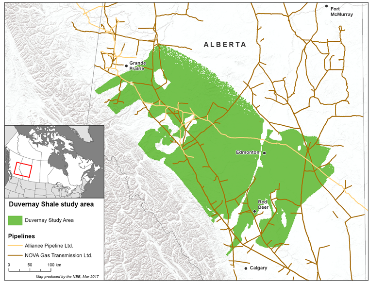
Figure 1. Location of the Duvernay Shale in Alberta and Canada
Source: NEB
Description:
This figure is a map that shows the location of the Duvernay Shale study area. Calgary, Alberta, is located just south of the study area's southern end while Grande Prairie, Alberta, is located at the study area's northwest end. The figure also shows the gas pipeline systems (Nova Gas Transmission Limited and Alliance Pipeline Limited) that run through the study area.
Methods
Supply costs for the Duvernay Shale’s marketable resources were estimated by finding the crude oil, natural gas and NGL prices required for a well to cover its costs and earn a 10% profit in each square-mile tract of the original Duvernay resource assessment. Gas supply costs were determined by holding some assumed oil prices constant. Oil supply costs were determined by holding some assumed natural gas prices constant. Well production varied by local geology and its oil, natural gas, and NGL contents were based on AGS maps of the in-place resource.Footnote 2
Costs included the cost to drill and hydraulically fracture a well (adjusted to the Duvernay’s local depth), operating costs, shipping costs to Alberta trading hubs, income taxes, royalties, and a carbon taxFootnote 3 on upstream and midstream emissions. Future revenues were discounted by 8% per year.Footnote 4 NGL prices were indexed to crude oil. Several different scenarios were run to estimate supply costs at different well costs and fixed crude oil and natural gas prices. Details are available in Appendix B.
Results and Observations
So far in 2017, Western Canadian light sweet oil prices at Edmonton have averaged about C$60/bbl and natural gas prices at Nova Inventory Transfer (NIT) about C$2.50/GJ. For 2018, the AER projects oil and natural gas prices will increase to about C$70/bblFootnote 5 and C$3.00/GJ, respectively.Footnote 6 Meanwhile, costs to develop shale gas and shale oil typically fall over time because operators learn from previous wells and increase efficiencies when drilling newer wells.
Altogether, once modeled, changes to well costsFootnote 7 and commodity prices significantly change the size of the Duvernay Shale’s economic resource (Tables 1 and 2 and Figures 3 to 6).Footnote 8 Tables 1 and 2 show the Duvernay Shale’s economic resources at C$60/bbl for crude oil and C$2.50/GJ for natural gas (in metric and imperial, respectively).
| C$60/bbl and C$2.50/GJ | C$70/bbl and C$3.00/GJ | |||||||
|---|---|---|---|---|---|---|---|---|
| Well Year | 2015 | 2016 | 2017 | 2018 | 2015 | 2016 | 2017 | 2018 |
| Oil (million m3) |
0.30 | 65.18 | 156.49 | 252.65 | 40.33 | 148.43 | 246.71 | 349.50 |
| Gas (billion m3) |
0.10 | 79.37 | 339.23 | 564.88 | 72.07 | 338.96 | 497.15 | 931.94 |
| NGLs (million m3) | 0.10 | 58.44 | 216.15 | 354.63 | 49.95 | 214.65 | 357.68 | 535.83 |
| C$60/bbl and C$2.50/GJ | C$70/bbl and C$3.00/GJ | |||||||
|---|---|---|---|---|---|---|---|---|
| Well Year | 2015 | 2016 | 2017 | 2018 | 2015 | 2016 | 2017 | 2018 |
| Oil (billion bbl) |
0.00 | 0.41 | 0.98 | 1.59 | 0.25 | 0.93 | 1.55 | 2.20 |
| Gas (Tcf) |
0.00 | 2.80 | 11.98 | 19.95 | 2.55 | 11.97 | 17.56 | 32.91 |
| NGLs (billion bbl) |
0.00 | 0.37 | 1.36 | 2.23 | 0.31 | 1.35 | 2.25 | 3.37 |
To summarize, at 2017 light sweet crude oil prices, natural gas prices, and well costs, the Duvernay Shale’s economic oil resource is 156 million cubic metres (m3) or 1.0 billion barrels; about one third of the Duvernay’s marketable oil resource. Meanwhile, the Duvernay Shale’s economic natural gas resource is 339 billion m3 (12.0 trillion cubic feet (Tcf)); 16% of the Duvernay’s marketable natural gas resource. The Duvernay Shale’s economic natural gas liquid (NGL) resource is 216 million m3 (1.4 billion barrels), about one fifth of the Duvernay’s marketable NGL resource.
Should well costs continue to fall and crude oil and natural gas prices modestly rise, the Duvernay Shale’s economic oil resource would increase to 350 million m3 (2.2 billion barrels), almost two thirds of the Duvernay’s marketable oil resources. The Duvernay Shale’s economic natural gas resource would increase to 932 billion m3 (32.9 Tcf), over 40% of its marketable natural gas resources. The Duvernay Shale’s NGL resource would increase to 536 million m3 (3.4 billion barrels), over half of the Duvernay’s marketable NGL resources.
Some areas of the Duvernay natural gas resource are economic at negative gas prices. This indicates that, in those areas, companies earn enough revenue from the oil and NGL production from a well that they can lose money on the natural gas production and still make a profit.
Overall, Duvernay Shale economics are very sensitive to declines in well costs as indicated by Figures 3 to 6. As well costs fall, increases to oil and gas prices cause economic resources to grow more rapidly than they would with higher well costs (i.e., the supply-cost curves flatten, and even small increases to prices can significantly increase the amount of economic resources).
Importantly, well production in the original NEB and AGS study was based on the average well drilled in 2016, and the size of 2017 and 2018 economic resources could be underestimated if well performance for newer wells has since improved. Improved technology often increases well performance and has been a key reason why supply costs of shale oil and shale gas production have been falling in North America over the past 10 years.
In particular, increases in well performance should have similar effects on supply costs as capital cost reductions of the same size (for example, a 20% increase in well production over its lifetime would have a similar effect on supply costs as a 20% reduction in costs to drill and hydraulically fracture that well). Thus, while the effects of increased well performance on supply costs were not modeled for this economic analysis, the reduction in supply costs from year to year can be a guide to how the economic resource could grow from 2017 to 2018 if the performance of new wells increases by 20% (or if there is a combination of cost reductions and improved well performance equivalent to a 20% reduction in capital costs).
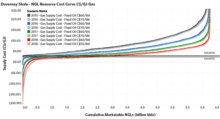
Figure 2. Supply-cost curves for the Duvernay Shale’s natural gas resources (imperial units only)
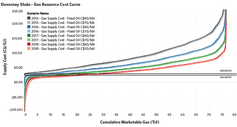
Note: the vertical axis is clipped at -C$10/GJ and C$25/GJ
Source: NEB
Description:
This figure is a chart showing the supply costs in C$/GJ for the Duvernay Shale's marketable gas resource. There are four sets of two curves, where each set represents a year from 2015 to 2018 while the pairs in each set represent fixed oil prices of C$60/bbl and C$70/bbl. Supply costs progressively lower with each year such that the resource's cost curves start flattening, and costs based on C$60/bbl oil are slightly higher than $70/bbl oil in each pair. Each cost curve starts with lower but steeply rising supply costs at the very low end of the gas resource. From the low end of the gas resource to the high end, the supply costs gently increase until the very high end of the gas resource, where supply costs are much higher and start steeply rising again.
Figure 3. Supply-cost curves for the Duvernay Shale’s crude oil resources (imperial units only)
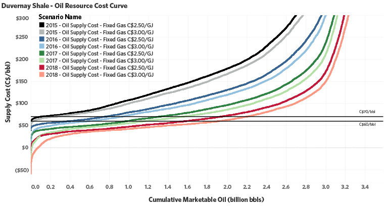
Note: the vertical axis is clipped at C$300/bbl
Source: NEB
Description:
This figure is a chart showing the supply costs in C$/bbl for the Duvernay Shale's marketable oil resource. There are four sets of two curves, where each set represents a year from 2015 to 2018 while the pairs in each set represent fixed gas prices of C$2.50/GJ and C$3.00/GJ. Supply costs progressively lower with each year and costs based on C$2.50/GJ oil are slightly higher than $3.00/GJ oil in each yearly pair. Each cost curve starts relatively flat at the low end of the resource, though grow steadily steeper towards the high end of the resource.
Figure 4. Supply-cost curves for the Duvernay Shale’s NGL resources (imperial units only)
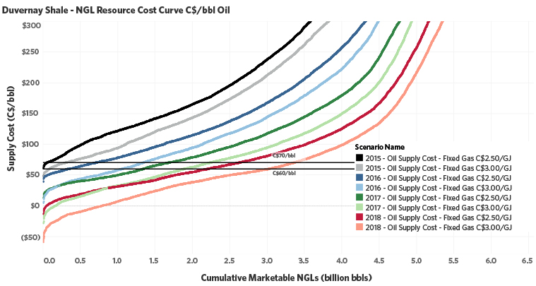
Note: the vertical axis is clipped at C$300/bbl
Source: NEB
Description:
This figure is a chart showing the supply costs in C$/bbl for the Duvernay Shale's marketable NGL resource. There are four sets of two curves, where each set represents a year from 2015 to 2018 while the pairs in each set represent fixed gas prices of C$2.50/GJ and C$3.00/GJ. Supply costs progressively lower with each year and costs based on C$2.50/GJ oil are higher than $3.00/GJ oil in each yearly pair. Supply costs steadily increase from the low end of the resource to the high end of the resource.
Figure 5. Supply-cost curves for the Duvernay Shale’s NGL resources (imperial units only)
Note: the vertical axis is clipped at -C$20/GJ and C$25/GJ
Source: NEB
Description:
This figure is a chart showing the supply costs in C$/GJ for the Duvernay Shale's marketable NGL resource. There are four sets of two curves, where each set represents a year from 2015 to 2018 while the pairs in each set represent fixed oil prices of C$60/bbl and C$70/bbl. Supply costs progressively lower with each year such that the resource's cost curves start flattening, and costs based on C$60/bbl oil are slightly higher than $70/bbl oil in each pair. Each cost curve starts with lower but steeply rising supply costs at the very low end of the gas resource. From the low end of the gas resource to the high end, the supply costs gently increase until the very high end of the gas resource, where supply costs are much higher and start steeply rising again.
Appendix A: Supply Cost Maps
Figure A1. Map of the Duvernay Shale’s crude oil supply costs at 2017 well costs and with the natural gas price constant at C$2.50/GJ
Duvernay Map - 2017 - Oil Supply Cost - Fixed Gas C$2.50/GJ
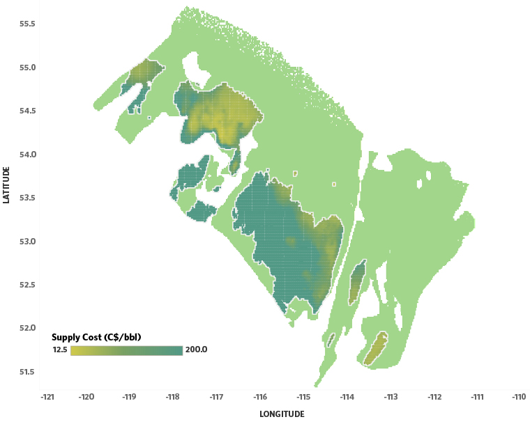
Note that the scale is limited to C$200/bbl (i.e., areas with supply costs higher than C$200/bbl will be mapped as if they have supply costs of C$200/bbl).
Source: NEB
Description:
This figure is a map that plots the the supply costs of the Duvernay Shale marketable oil resource over the study area (2017 well costs with gas prices fixed at C$2.50/GJ). The marketable oil is most economic in pockets in the north central part of the Duvernay Shale basin, and in pockets in the far southeast. The least economic oil is found on the Duvernay Shale's southwest side.
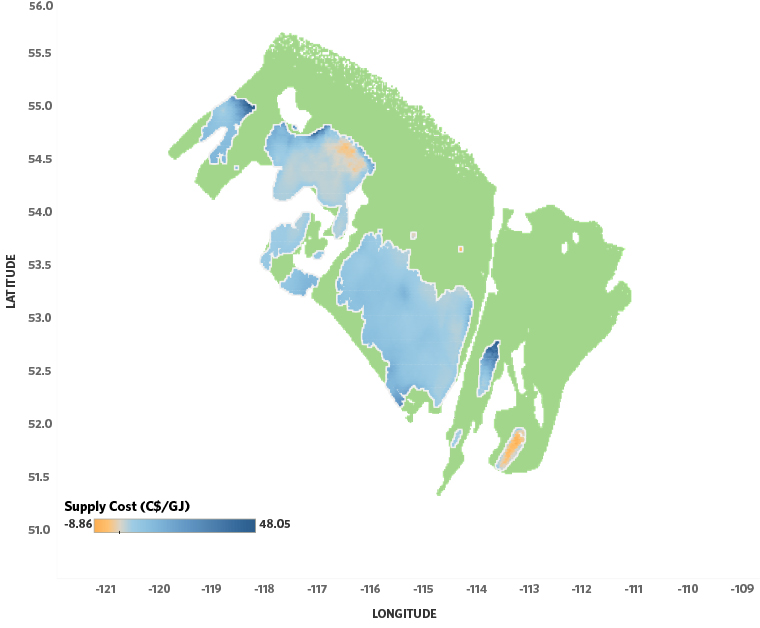
Figure A2. Map of the Duvernay Shale’s natural gas-supply costs at 2017 well costs and with the light sweet crude oil price constant at C$60/bbl
Duvernay Map - 2017 - Gas Supply Cost - Fixed Oil C$60/bbl
Source: NEB
Description:
This figure is a map that plots the the supply costs of the Duvernay Shale marketable gas resource over the study area (2017 well costs with oil prices fixed at C$60/bbl). The marketable gas is most economic in pockets in the north central part of the Duvernay Shale basin, and in a pocket to the far southeast.
Figure A3. Map of the Duvernay Shale’s crude oil supply costs at 2018 well costs and with the natural gas price constant at C$3.00/GJ.
Duvernay Map - 2018 - Oil Supply Cost - Fixed Gas C$3.00/GJ
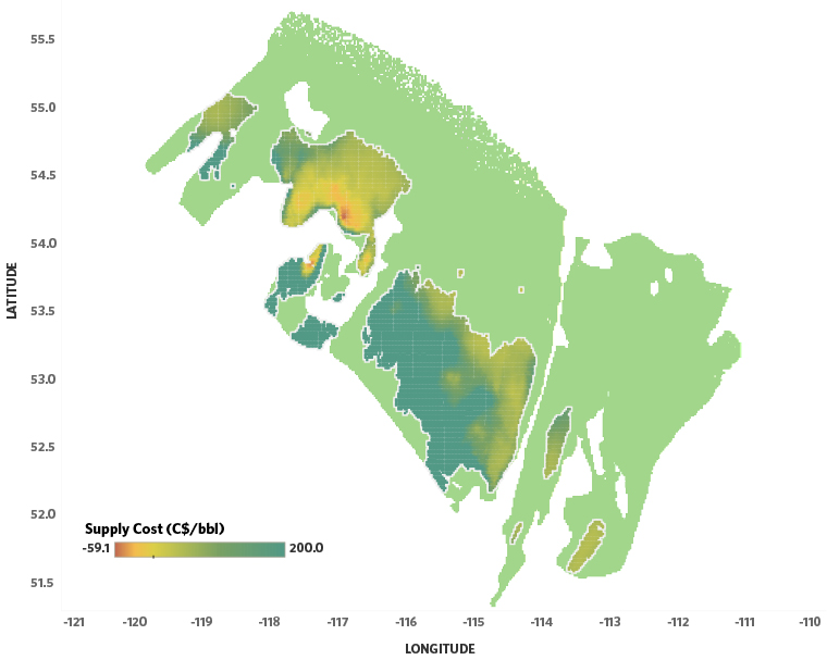
Note that the scale is limited to C$200/bbl (i.e., areas with supply costs higher than C$200/bbl will be mapped as if they have supply costs of C$200/bbl).
Source: NEB
Description:
This figure is a map that plots the the supply costs of the Duvernay Shale marketable oil resource over the study area (2018 well costs with gas prices fixed at C$3.00/GJ). The marketable oil is most economic in pockets in the north central part of the Duvernay Shale basin, and in pockets in the southeast. The least economic oil is found on the Duvernay Shale's southwest side.
Figure A4. Map of the Duvernay Shale’s natural gas-supply costs at 2018 well costs and the light sweet crude oil price constant at C$70/bbl
Duvernay Map - 2018 - Gas Supply Cost - Fixed Oil C$70/bbl

Source: NEB
Description:
This figure is a map that plots the the supply costs of the Duvernay Shale marketable gas resource over the study area (2018 well costs with oil prices fixed at C$70/bbl). The marketable gas is most economic in pockets in the north central part of the Duvernay Shale basin, and in pockets to the far southeast.
Appendix B: Detailed Methods
Key Assumptions
Well production is based on existing technology, current trends in development, and limited amounts of historical production. No detailed analyses of technological advancements have been performed for this study. Recoveries and levels of development could be different in the future as technology advances and the play matures.
Study Area
As in the original study, the study area was broken down into tractsFootnote 9 of approximately one-square mile in size. Some tracts were excluded from the analysis because they were considered unlikely to be developed; such as where the Duvernay Shale is less than 10 m thick, is underpressuredFootnote 10, where its mapped in-place natural gas contents are less than 50 m3 of volume per m2 of area, and where oil contents were more than 2 000 barrels per million cubic feet of gas. Only 27 819 square kilometres (km2) of the full 108 244 km2 assessed by the AER for in-place resources (or 10 803 of the study area’s 42 012 square-mile tracts) were included after these criteria were applied (Figure B1).
Figure B1. Duvernay Shale study area and assessed study area
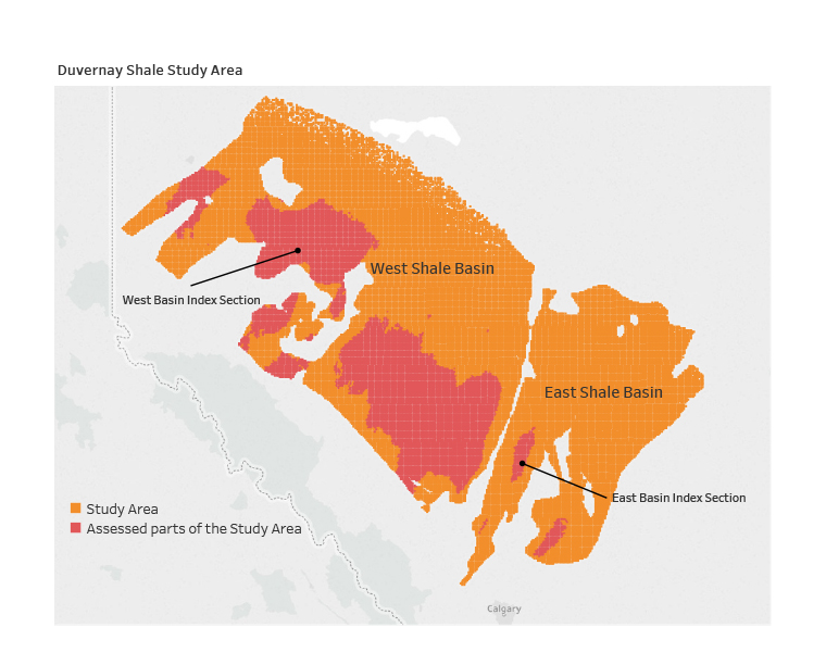
Source: NEB and AGS
Description:
This figure is a map that shows the study area, as well as what areas were assessed and what were excluded because of geological cutoffs. The southeast third of the Duvernay Shale basin is called the East Shale Basin and the northwest two-thirds is called the West Shale Basin. Most of the assessed area is located in the southwest half of the West Shale Basin while only three small parts of the East Shale Basin were assessed. This figure also shows the locations of the two index sections used for the assessment.
Production-curve Modeling and Estimation of Resources
Please see Appendix B of the NEB and AGS resources report.
Supply Costs
Each tract’s supply costs for marketable crude oil, natural gas, and NGLs were estimated by determining the crude oil and natural gas pricesFootnote 11 needed so that a typical development well could earn a 10% rate of return once its net present costs were subtracted from its net present revenues. Natural gas supply costs were determined using a series of fixed crude oil prices (from C$50/bbl to C$100/bbl in $10 increments) while crude oil supply costs were determined using a series of fixed natural gas prices (from C$2.00/GJ to C$4.50/GJ in $0.50 increments). Natural gas prices were assumed to be C$/GJ at NITFootnote 12, and crude oil prices were assumed to be light, sweet, crude oil in C$/bbl at Edmonton. All costs were in Canadian dollars, so no exchange rate was used. All prices and costs used were in 2017 dollars.
The marketable production for a typical development well in a tract was estimated in the same way that a tract’s estimated ultimately recoverable (EUR) marketable production was estimated, except that the well’s horizontal leg length was increased to 2.5 km from 1.6 km. Thus the development well’s estimated supply costs could be applied to the tract’s EURs of marketable natural gas, crude oil, and NGLs.
Monthly revenues for a development well in a tract were estimated from:
- The heat content of the monthly marketable natural gas (including unrecovered NGLs) and marketable ethane;
- The volumes of monthly NGLs other than ethane, as indexed to the crude oil price
(40% for propane, 70% for butanes, and 105% for pentanes plus); and - The volume of monthly crude oil, with a 5% premium to the crude oil price because of the high demand for condensate and very light oil to be used as diluent in western Canada.
Costs for a development well in each tract were determined on the basis of:
- The capital cost of drilling and completing a well in a tract, as based on the equation for the Drilling and Completion Cost Allowance (C*) of Alberta’s Modernized Royalty Framework (MRF). Each well was assumed to have a vertical depth measured to the top of the Duvernay Formation in the tract and a 2.5 km horizontal leg. Each well was also assumed to use 600 tonnes of proppant.Footnote 13 The capital cost was assumed to include tying the well into local natural gas gathering pipelines. The capital cost of abandoning the well at the end of its productive life ($100 000) was also included. Three well cost scenarios (as based on reported costs by industry from 2015, 2016, and 2017) were used to find how changing capital costs can alter supply costs, including the shape of the resource’s cost curve. An additional, future well cost scenario was used to model how supply costs change if well costs continue to fall.
- 2015 well costs were assumed to be 125% of estimated C*;
- 2016 well costs were assumed to be 100% of estimated C*;
- 2017 well costs (or current well costs) were assumed to be 80% of estimated C*; and
- 2018 well costs (or future well costs if companies continue to increase operational efficiencies) were assumed to be 64% of estimated C* (i.e., 20% less than 2017 well costs).
- This study assumes 2015 through 2018 well costs would not vary with changes to calculated supply costs nor with the fixed crude oil and natural gas prices the supply costs are paired with (e.g., a well that is marginally economic when crude oil is C$60/bbl and natural gas C$2.50/GJ would cost the same as a well when crude oil is C$70/bbl and gas C$3.00/GJ). In reality, higher crude oil and natural gas prices cause cost inflation because activity increases across the crude oil and natural gas sector. Thus, well costs and their associated supply costs would likely be higher than estimated for some of the higher crude oil and natural gas prices in this study (e.g., fixed crude oil prices at C$100/bbl and fixed gas prices at C$4.50/GJ).
- No petroleum land rights costs, because prospective rights were largely purchased for prospective areas before 2017 and these costs are already sunk.
- No geological and geophysical costs.
- Monthly operating costs, with fixed monthly costs of $2 000/month plus variable costs of $0.85 per thousand cubic feet (mcf) for raw natural gas and $7.00/barrel for crude oil.
- Monthly shipping costs of $0.25/GJ for marketable natural gas to NIT and ethane to Edmonton, and $2/barrel for other NGLs and crude oil to Edmonton.
- Monthly royalties as determined by Alberta’s MRF, including pre-payout, payout, and mature royalty rates.Footnote 14 Payout and mature royalty rates were based on Alberta Energy’s royalty equations, which consider crude oil and natural gas prices and production rates. The C* Drilling and Completion Cost Allowance, which determines how much revenue a producer can collect from a well before the pre-payout period ends, was estimated by the well depth, horizontal leg length, and proppant used (assuming 600 tonnes). C* was then adjusted upward by 25% to include the Alberta’s Emerging Resources Program, which allows companies to increase their C* allowance by 50% to 100% for the first 15% of wells drilled on a prospect.
- Monthly corporate income taxes, both federal (15%) and provincial (12%), including deductions for operating costs, shipping costs, royalties, and carbon taxes.
- Deductions include the federal Capital Development Expense as based on the capital cost of the well.Footnote 15
- A monthly, escalating carbon tax was applied to dry natural gas consumed for natural gas processing and transmission (0.117 tonnes of carbon dioxide equivalent (CO2e)/mcf). Fuel gas for wellsite operations, however, was excluded because Alberta’s carbon levy currently does not apply to it. The carbon tax was also applied to crude oil and NGLs shipped by pipeline to Edmonton (0.000414 kgCO2e/bbl/km) as based on GHG-intensity estimates for shipping synthetic crude oil.Footnote 16 The carbon tax was assumed to start at $20/tonne and escalate to a maximum of $50/tonne over 5 years. A carbon tax of $20/tonne was added to the capital costs as based on 300 000 litres (L) of gasoline (2.31 kgCO2/L) used for drilling and well completion as well as trucking of equipment, personnel, supplies, and flowback water handling.
The financial assumptions included:
- A 10% rate of return.
- An 8% discount rate (based on the cost of capital).
- Constant crude oil and natural gas prices, and no cost inflation applied to operating costs and shipping costs.
- For determining EURs, wells would be abandoned after 40 years of production.
- No corporate overhead.
- Date modified: