ARCHIVED – Canada’s Energy Future 2017 Supplement: Natural Gas Production – Appendix
This page has been archived on the Web
Information identified as archived is provided for reference, research or recordkeeping purposes. It is not subject to the Government of Canada Web Standards and has not been altered or updated since it was archived. Please contact us to request a format other than those available.
Canada’s Energy Future 2017 Supplement: Natural Gas Production [PDF 2729 KB]
Appendix Data and Figures [EXCEL 10014 KB]
January 2018
Copyright/Permission to Reproduce
ISSN 2369-1479
Table of Contents
Appendix A
A1 – Method (Detailed Description)
Canadian natural gas production from 2017 to 2040 will consist of conventional and tight gas production from the WCSB with contributions from Atlantic Canada, Ontario, coalbed methane (CBM) production from Alberta, and shale gas production from Alberta and B.C. Analysis in this report includes trends in well production characteristics and resource development expectations – used to develop parameters that define future natural gas production from the WCSB. Different approaches were used for other regions of Canada where production is sourced from a smaller number of wells.
A1.1 WCSB
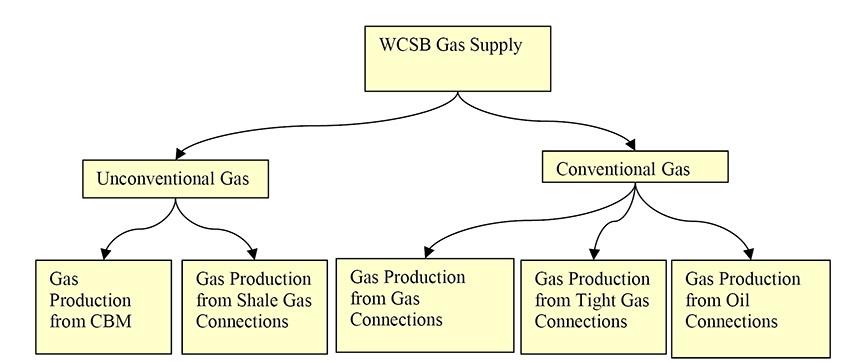
To assess gas production for the WCSB, gas production was split into five type categories as shown in Figure A1.1.
Figure A1.1 - WCSB Major Gas Production Categories
Description:
This illustration shows the categories of western Canada natural gas production. Natural gas is broken down by either unconventional or conventional gas. Unconventional gas is then broken down by type of gas – either CBM or shale. Conventional is also broken down by type of gas – either tight gas, non-tight gas, or solution gas.
The method to determine gas production associated with conventional gas wells (including tight gas), CBM wells, and shale gas wells is described below. Production decline analysis on historical production data was used to determine parameters that define future performance. The method to determine gas production related to oil wells (solution gas) is described in Section A1.1.2 of this appendix.
A1.1.1 Groupings for Production Decline Analysis
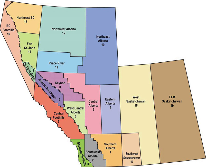
Different groupings by type of gas well were made to assess well performance characteristics. Conventional, tight, and shale gas wells were grouped geographically on the basis of the Petrocube areas in Alberta, B.C., and Saskatchewan, as shown in Figure A1.2. These wells were also grouped by geological zone. In this analysis, gas production from the Montney Formation is separate from the other tight gas sources.
Figure A1.2 - WCSB Area Map
Description:
This map shows the western Canadian natural gas areas. There are three areas in northeast British Columbia, 12 areas in Alberta, and three areas in Saskatchewan.
Within each PetroCUBE area and zone, gas wells were grouped by year, with all wells existing prior to 1999 forming a single group, and separate groups for each year from 1999 through 2040.
CBM wells in Alberta were also grouped primarily by zone into three categories:
- Horseshoe Canyon Main Play
- Mannville CBM, and
- Other CBM
Within each of the three categories of CBM resources, wells were also grouped by well year. For the Horseshoe Canyon Main Play and Other CBM categories, there is a single grouping for all wells existing prior to 2004, and separate groupings for each year thereafter. For Mannville CBM, a single grouping was made for all wells existing prior to 2006, and separate groupings for each following year.
In total there are about 150 gas resource groupings representing Western Canada, each with its own set of decline parameters for each year.A1.1.2 Method for Existing Wells
The method applied to make the gas production projections for existing wells differs from what is done to project production for future wells. For existing wells, production decline analysis on historical production data is done on each grouping (gas type/Petrocube area/geological zone and by well year) to develop two sets of parameters.
- Group production parameters-- describing production expectations for the entire gas resource grouping.
- Average well production parameters - describing production expectations for the average gas well in the grouping.
The method for the production decline analysis on existing wells is described below. The group production parameters and average well production parameters resulting from this analysis are contained in Appendices A.3 and A.4, respectively.
In the model, the group production parameters are used to make the production projection for existing wells. For each of these groupings, a data set of group marketable production history is created. The data sets for group marketable production are generated as follows:
- Raw well production for gas connections in each grouping is summed by calendar month getting total group raw production by calendar month.
- The total group raw production by calendar month is multiplied by an average shrinkage factor that applies to the grouping and divided by the number of days in each month to get total monthly marketable gas production and marketable gas production rate (MMcf/d) for each calendar month.
- Using this data set, plots of total daily marketable production rate versus total cumulative marketable production are generated for each grouping.
The data sets for average well production history are created as follows.
- The raw well production by month for each connection in the grouping is put in a data base.
- For each entry of production month for each well, a value of normalized production month is calculated as the number of months between the month the connection began producing and the actual production month (this is the normalized production month).
- The raw production for wells in the grouping is summed by normalized production month and then multiplied by the average shrinkage factor that applies to the grouping, providing total marketable production by normalized production month.
- The marketable production for normalized production month is then divided by the average number of days in a month, or 30.4375, giving the production rate for the average well in the grouping by normalized production month.
- Using this data set, daily marketable production rate versus cumulative marketable production for the average well were generated for each grouping.
For conventional gas wells, the following procedures are applied in performing production decline analysis using the group and average well historical production data sets:
- Production Decline Analysis for the Pre-1999 Wells
In each grouping, the group rate versus cumulative production plot for the grouping of gas wells on production prior to 1999 is the first to be evaluated. In all groupings a stable exponential decline for the past several years was exhibited. The group plot for all the wells prior to 1998 yields a current marketable production rate, a stable decline rate applicable to future production, and a terminal decline if seen fit.
- Production Decline Analysis for 1999 - 2016 Wells
After the initial aggregate well year is evaluated for a grouping, each year is evaluated in sequence, from 1999 through 2016.
a. Production Decline Analysis for the Average Well:
For each well year, the rate versus cumulative production plot for the average well is evaluated first to establish the following parameters that describe the production profile of the average well over the entire productive life:
- Initial Production Rate
- First Decline Rate
- Second Decline Rate
- Months to Second Decline Rate- usually around 18 months
- Third Decline Rate
- Months to Third Decline Rate- usually around 45 months
- Fourth Decline Rate
- Months to Fourth Decline Rate- usually around 100 months.
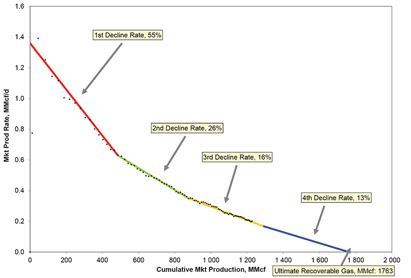
Figure A1.3 shows an example of the plots used in evaluation of average well performance, and the different decline rates that are applied to describe the production.
Figure A1.3 – Example of Average Well Production Decline Analysis Plot
Source and Description:
Source:
NEB analysis of Divestco Geovista well production data
Description:
This graph shows an example of a decline curve for an average natural gas well. The initial production rate is 1.39 MMcf/d. For the first seven months the well production rate has a decline rate of 55%. The second decline rate is 26%, the third is 16%, the fourth is 13% and the final decline rate is 5%. Total well production is 1 763 MMcf.
For the earlier well years, the available data is usually sufficient to establish all of the above parameters. For more recent well years, the duration of historical production data becomes shorter and the parameters describing the later life decline performance must be taken from that determined for earlier well years. In the example shown in Figure A1.3, the available data is sufficient to determine parameters defining the first, second, and third decline periods for the well, but the parameters defining the fourth decline period must be assumed based on the analysis of earlier well years.
It is assumed that, unless the historical data for the well year indicates otherwise, the fourth decline rate will equal the terminal decline rate for the grouping established through evaluation of all pre-1999 wells, and that period of the terminal decline rate will commence after 120 months of production.
The decline parameters determined in this manner for average wells are available in Appendix A4.
b. Production Decline Analysis for the Group Data:
Once the performance parameters for the average well are established, the procedure focuses on evaluation of group performance parameters.
As a first step, the average well performance parameters are combined with the known 12-month well schedule to calculate the expected group performance. This is plotted with the actual group performance data. If the data calculated from average well performance data does not provide a good match with the actual historical production data for the group, then the average well parameters may be revised until a good match is obtained between calculated group production data (from average well data) and actual group production data. An example of the group plots described here is shown in Figure A1.4.
Figure A1.4 – Example of Group Production Decline Analysis Plot
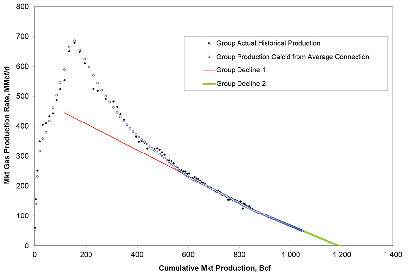
Source and Description:
Source:
NEB analysis of Divestco Geovista well production data
Description:
This graph shows an example of a decline curve for a group of wells. The peak production rate occurs in month 13 and is 679.9 MMcf/d.
The following group performance parameters are determined from the group plot:
- Production Rate as of month one
- First Decline Rate
- Second Decline Rate (if applicable)
- Months to Second Decline Rate (if applicable)
- Third Decline Rate (if applicable)
- Months to Third Decline Rate (if applicable)
- Fourth Decline Rate (if applicable)
- Months to Fourth Decline Rate (if applicable)
In the earlier well year groupings (2001, 2002, etc.), the actual group data is usually stabilized by the current date at or near the terminal decline rate established via the pre-1999 aggregate grouping. In these cases a single decline rate sufficiently describes the entire remaining productive life of the grouping. In these cases the expected performance calculated from average well data has little influence over determination of the group parameters.
In later well years (2015, 2016, etc.) actual group production history data cannot provide a good basis upon which to project future production. In these cases the expected performance calculated from average well data is vital to establishing the current and future decline rates.
Group performance parameters determined in this manner are available in Appendix A3.
The production decline analysis procedure described above is also applied to the CBM groupings and shale gas. Mannville CBM connections have a different performance profile than the other gas resources in the WCSB. While gas wells for all other groupings can be described by an initial production rate that declines in a relatively predictable manner, Mannville CBM connections go through a dewatering phase with gas production increasing over a period of months to a peak rate. After the peak rate is reached decline will occur. Thus a slightly different set of parameters is used to describe performance of the average well for Mannville CBM, with initial production rate being replaced by “Months to Peak Production” and “Peak Production Rate”.
The shorter production history of shale gas makes it more difficult to establish long-term decline rates based on historical data. Nevertheless, decline rates that describe the full productive life of shale gas wells are still estimated based on the NEB’s view of ultimate gas recovery for the average well.
A1.1.3 Method for Future Wells
For future wells, production is estimated based on the number of projected wells and the expected average performance characteristics of those wells. The drilling projection is used to estimate the number of future gas wells. Historical trends in average well performance parameters, obtained from production decline analysis of existing gas wells, are used to estimate average well performance parameters for future well years.
A1.1.3.1 Performance of Future Wells
The performance of future wells is obtained in each grouping by extrapolating the production performance trends for average wells in past years. The performance parameters estimated are initial productivity of the average well and the associated decline rates.
In many groupings there are trends of decreasing or increasing initial productivity for the average gas well. Figure A1.5, which shows the initial production rate over time for tight gas wells in the Alberta Deep Basin Upper Colorado grouping. The IP was trending down until about 2006 when horizontal drilling and multi-stage hydraulic fracturing technologies started taking off, which increased the IP over the last decade in this grouping. The initial production rate for future gas wells is estimated by extrapolating the trend in each grouping, and are adjusted if there are any other assumptions such as technological or resource changes. Historical and projected initial productivity values for the average well for all groupings are contained in Appendices A3 and A4.
Figure A1.5 – Example of Average IP by Year – Alberta Deep Basin Upper Colorado Tight Grouping
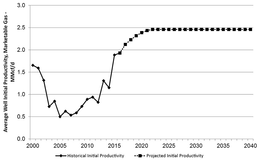
Source and Description:
Source:
NEB analysis of Divestco well production data
Description:
This graph shows the IP by well year for the Alberta Deep Basin tight, upper Colorado grouping. Wells drilled in 2000 had an average IP of 1.65 MMcf/d. Wells drilled in 2005 had the lowest average IP rate at 0.50MMcf/d. Wells drilled in 2016 had an average IP of 1.93 MMcf/d. The average IP of wells is projected to increase to 2.46 MMcf/d in 2022 and stay at that level to the end of 2040.
The key decline parameters impacting the near term are the first decline rate, second decline rate, and months to second decline rate. Figure A1.6 shows the historical and projected values of these key decline parameters for the average well in the Alberta Deep Basin Mannville Tight grouping. As shown in Figure A1.6, trends seen in the decline parameters in past years are used to establish these key parameters for future years.
Figure A1.6 – Example of Key Decline Parameters Over Time – Alberta Deep Basin Mannville Tight Grouping
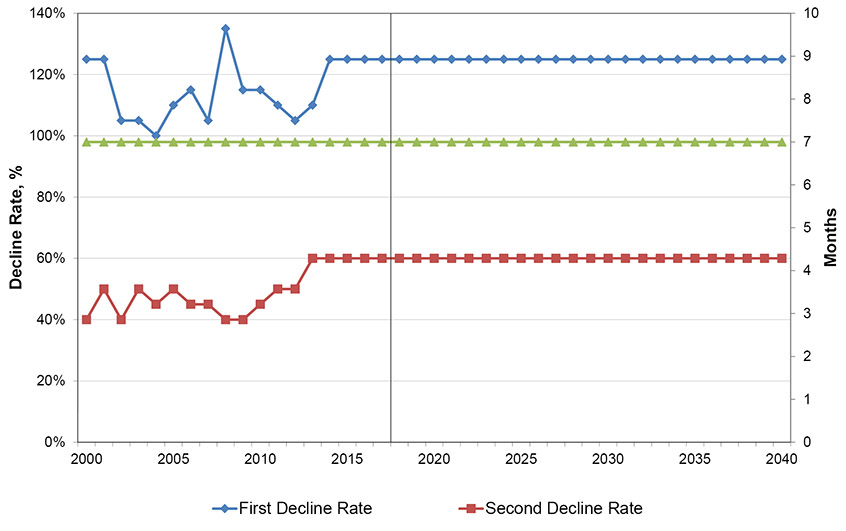
Description:
This graph shows the first and second decline rates by well year for the Alberta Deep Basin tight Mannville grouping. From 2000 to 2016 the first decline rate ranged between 100% and 135%. The projected rate is 125% for all well years. From 2000 to 2016 the second decline rate ranged between 40% and 60%. The projected rate is 60% for all well years. The months to the second decline rate is steady at seven.
A1.1.3.2 Number of Future Wells
Figure A1.7 shows the method for projecting the number of gas wells for each year over the projection period. The key inputs are amount of re-investment of revenue and the drill day cost. Adjustments to these two key inputs can significantly change the drilling projections. The values projected for the other inputs are estimated from an analysis of historical data.
The Board projects an allocation of gas drill days for each of the groupings. The allocation fractions are determined from historical trends, recent estimates of supply costs, and the Board’s view of development potential for the groupings. The allocation fractions reflect the historical trends of an increasing focus on the deeper formations located in the western side of the basin, increasing interest in tight gas and gas shales in B.C. and Alberta, and further development of liquids rich/wet natural gas. Tables of drill days by year by grouping for each case are in Appendices B1.1 – B1.6.
The number of gas wells drilled in each year is calculated by dividing the drill days targeting each resource grouping by the average number of days it takes to drill a well. Future drill days per well for each grouping are based on historical data, and any assumptions on drilling efficiency or resource changes. Tables of wells by year by grouping for each case are in Appendices B2.1 – B2.6.
Figure A1.7 – Flowchart of Drilling Projection Method
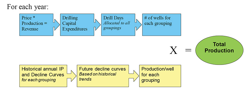
Description:
This illustration shows how total production is calculated. For a given year, price multiplied with production equals revenue. An assumed amount of that revenue is used as drilling capital expenditures. The cost per drill day for that year is divided into the drilling expenditures to get the total number of drill days, which are then allocated to each of the gas groupings to get the number of wells per grouping given the number of drill days to drill a well in each grouping. To get production per well the historical IP and decline curves for each grouping are used to get future IP and decline curves for the given year. Finally, the number of wells multiplied with the production per well equals the production per grouping and total production is the sum of production from all groupings.
A1.1.4 Solution Gas
Solution gas is gas produced from oil wells in conjunction with the crude oil and currently accounts for over 10% of total marketable gas production in the WCSB. Solution gas analysis is by Petrocube area and is projected by using historical trends and projected conventional, tight, and shale oil production by province (see EF2017 Supplement: Conventional, Tight, and Shale Oil Production). The projected solution gas production is deemed to represent all solution gas production (i.e. production from both existing and future oil wells).
A1.1.5 Yukon and Northwest Territories
No production from the Mackenzie Delta and elsewhere along the Mackenzie Corridor is included over the projection, as lower prices have rendered production uneconomic. The Norman Wells field produces small amounts of gas that serve local purposes and is not tied into the North American pipeline grid. Cameron Hills production ceased in February 2015.
A1.2 Atlantic Canada
For producing wells from offshore Nova Scotia, production profiles are based on the seasonal performance of the two producing projects. No additional infill wells are assumed for the producing fields over the projection period. Production from the Deep Panuke development started in fall 2013, but has since turned seasonal.
Onshore production from the McCully Field in New Brunswick was connected into the regional pipeline system at the end of June 2007 and now operates on a seasonal basis.
Shale gas potential exists in New Brunswick and Nova Scotia, however, provincial policies currently prohibit hydraulic fracturing which is required for shale gas development. It is assumed these policies do not change over the projection period.
A1.3 Other Canadian Production
A minor remaining amount of Canadian production is from Ontario. Production from Ontario is projected by extrapolation of historical production volumes. Shale gas potential exists in Quebec, however, provincial policies currently prohibit hydraulic fracturing which is required for shale gas development. It is assumed these policies do not change over the projection period.
Appendix A2 - Production Parameters - Results
A2.1 WCSB
A2.1.1 Production from Existing Gas Wells
The future production of existing wells of the resource groupings comprising conventional (including tight gas), and unconventional (including shale gas and CBM), and all solution gas was determined via the production analysis procedures described in Appendix A1. The decline parameters for these groupings are the same for all cases.
The parameters describing future production for all of these groupings are the production rate as of December 2016 and as many as four future decline rates that apply to specified time periods in the future. For the older wells where production appears to have stabilized at a final decline rate, only one future decline rate is needed to describe future group deliverability. For newer wells, the decline rate that applies over future months changes as the group performance progresses towards the final stable decline period. For these newer wells, three or possibly four different decline rates have been determined to describe future performance.
The projected production from existing wells represents the production that would occur from the WCSB if no further gas wells started producing after December 2016. Production from future gas wells supplements the declining production from existing wells.
A2.1.2 Production from Future Gas Wells
Production associated with future gas wells is calculated for each resource grouping using estimates for production performance of the average well and the number of wells in future years. The parameters associated with both of these inputs are discussed in the sections below.
While past projections for existing gas wells have enjoyed a high degree of accuracy, the certainty associated with the projections for future gas wells is less. The key uncertainties are the level of gas drilling that will occur and the production levels of wells. The high and low price cases aim to address the uncertainty inherent in the gas drilling projections.
A2.1.2.1 Performance Parameters for Future Average Gas Wells
The production decline analysis procedures described in Appendix A.1 provide the basis for establishing performance parameters for future gas wells. The trends seen in average well performance for the various groupings of existing wells are used to make an estimate of performance parameters for future gas wells.
With respect to initial productivity of the average gas well, the overall trend for the WCSB is shown in Figure A2.1. After decreases in initial productivity over 2001 to 2006, the trend reversed upward for 2007, remained fairly stable through 2009, and continued upward through to 2015 as higher initial productivity rates from tight gas and shale gas wells began to represent a growing share of the wells drilled in a year. Initial productivity over the projection is almost flat primarily due to holding the rates constant for most gas wells.
Figure A2.1 - WCSB Production-Weighted Average IP by - Reference Case

Source and Description:
Source:
NEB Analysis of Divestco Well Production Data
Description:
This graph shows the average IP by well year for all natural gas wells drilled in western Canada, weighted by production. Wells drilled in 2000 had an average IP of 1.17 MMcf/d. Wells drilled in 2006 had the lowest average IP rate at 0.54 MMcf/d. Wells drilled in 2016 had an average IP of 2.21 MMcf/d. The average IP of wells is projected to increase to 2.35 MMcf/d in 2040.
Table A2.1 shows the historical production-weighted average IP for wells by area by year. Appendices A3 and A4 provide historical and projected performance parameters for all groupings.
The performance parameters projected are the same in all cases assessed in this report. Variance between the cases is affected by applying different levels of gas drilling activity as discussed further in Section A2.1.2.2 of this appendix.
A2.1.2.2 Number of Future Gas Wells
The projected number of wells by year and the projected production performance of the average wells in those years determine projected production of future gas wells. To determine the number of future gas wells, projections of gas drilling activity by grouping are made.
Volatile and unpredictable market conditions are expected to be the primary influences on gas drilling activity. As a result, there is a high degree of uncertainty in the gas drilling activity that could occur over the projection period. The High Price Case and Low Price Case reflect a range of market conditions that may occur over the projection period. Figure A2.2 shows the total projected number of gas wells by year by case.
Projected annual gas wells and drilling days for each grouping are provided in Appendices B1.1 to B1.6 and B2.1 to B2.6.
Figure A2.2 – WCSB Gas Wells by Case
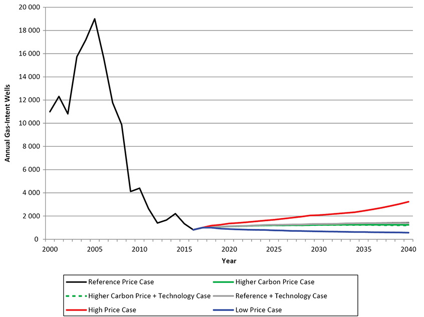
Description:
This graph shows the projected number of natural gas wells by year for all six cases. In 2000 there were 10 993 wells, and that increased and peaked in 2005 at 18 998 wells. Since then the number of wells has decreased and was at 813 in 2016. In the Reference Case the number of wells is projected to increase to 1 428 in 2040. In the Higher Carbon Price Case the number of wells is projected to increase to 1 243 in 2040. In the Higher Carbon Price and Technology Case the number of wells is projected to increase to 1 198 in 2040. In the Reference and Technology Case the number of wells is projected to increase to 1 395 in 2040. In the High Price Case the number of wells is projected to increase to 3 231 in 2040. In the Low Price Case the number of wells is projected to decrease to 569 in 2040.
A2.2 Atlantic Canada, Ontario, and Quebec
As indicated in Appendix A1, production from Atlantic Canada and Ontario is based on extrapolation of prior trends. No additional wells over the projection period are assumed to be drilled that would contribute to production at this time.
Marketable production from the Deep Panuke development started in fall 2013. Deep Panuke has begun producing seasonally in the winters, however incursion of water into the reservoir could adversely impact the amount of natural gas recoverable over the lifetime of the project. In this report offshore natural gas production in Nova Scotia declines steadily over the projection period and production ceases in 2021 for both the Deep Panuke and Sable projects.
Provincial policy in New Brunswick and Nova Scotia currently prohibits hydraulic fracturing which is required for shale gas development. It is assumed that these policies do not change and no additional onshore gas wells are drilled over the projection period. Ontario production continues to decline with no additional drilling expected over the projection period.
Provincial policy in Quebec currently prohibits hydraulic fracturing which is required for shale gas development. It is assumed that these policies do not change and no additional gas wells are drilled over the projection period.
Appendix A3 – Groupings and Decline Parameters for Existing Wells
Table A3.1 – Formation Index
| Formation | Abbreviation | Group Number |
|---|---|---|
| Tertiary | Tert | 02 |
| Upper Cretaceous | UprCret | 03 |
| Upper Colorado | UprCol | 04 |
| Colorado | Colr | 05 |
| Upper Mannville | UprMnvl | 06 |
| Middle Mannville | MdlMnvl | 07 |
| Lower Mannville | LwrMnvl | 08 |
| Mannville | Mnvl | 06;07;08 |
| Jurassic | Jur | 09 |
| Upper Triassic | UprTri | 10 |
| Lower Triassic | LwrTri | 11 |
| Triassic | Tri | 10;11 |
| Permian | Perm | 12 |
| Mississippian | Miss | 13 |
| Upper Devonian | UprDvn | 14 |
| Middle Devonian | MdlDvn | 15 |
| Lower Devonian | LwrDvn | 16 |
| Siluro/Ordivician | Sil | 17 |
| Cambrian | Camb | 18 |
| PreCambrian | PreCamb | 19 |
Table A3.2 – Grouping Index
| Area Name | Area Number | Resource Type | Resource Group |
|---|---|---|---|
| CBM Area | 00 | CBM | Main HSC |
| CBM Area | 00 | CBM | Mannville |
| Southern Alberta | 01 | Conventional | Tert;UprCret;UprColr |
| Southern Alberta | 01 | Conventional | Colr |
| Southern Alberta | 01 | Conventional | Mnvl |
| Southern Alberta | 01 | Tight | UprColr |
| Southwest Alberta | 02 | Conventional | Tert;UprCret;UprColr |
| Southwest Alberta | 02 | Conventional | Colr |
| Southwest Alberta | 02 | Conventional | MdlMnvl;LwrMnvl |
| Southwest Alberta | 02 | Conventional | Jur;Miss |
| Southwest Alberta | 02 | Conventional | UprDvn |
| Southwest Alberta | 02 | Tight | UprColr |
| Southwest Alberta | 02 | Tight | Colr |
| Southwest Alberta | 02 | Tight | LwrMnvl |
| Southern Foothills | 03 | Conventional | Miss;UprDvn |
| Eastern Alberta | 04 | Conventional | UprCret;UprColr |
| Eastern Alberta | 04 | Conventional | Colr;Mnvl |
| Eastern Alberta | 04 | Tight | UprColr |
| Eastern Alberta | 04 | Shale | Duvernay |
| Central Alberta | 05 | Conventional | Tert;UprCret |
| Central Alberta | 05 | Conventional | Colr |
| Central Alberta | 05 | Conventional | Mnvl |
| Central Alberta | 05 | Conventional | Miss;UprDvn |
| Central Alberta | 05 | Tight | Colr |
| Central Alberta | 05 | Tight | Mvl |
| Central Alberta | 05 | Tight | Montney |
| Central Alberta | 05 | Shale | Duvernay |
| West Central Alberta | 06 | Conventional | Tert |
| West Central Alberta | 06 | Conventional | UprCret;UprColr |
| West Central Alberta | 06 | Conventional | Mnvl |
| West Central Alberta | 06 | Conventional | LwrMnvl; Jur |
| West Central Alberta | 06 | Conventional | Miss |
| West Central Alberta | 06 | Conventional | UprDvn |
| West Central Alberta | 06 | Tight | Colr |
| West Central Alberta | 06 | Tight | Mnvl |
| West Central Alberta | 06 | Tight | Montney |
| West Central Alberta | 06 | Shale | Duvernay |
| Central Foothills | 07 | Conventional | UprColr |
| Central Foothills | 07 | Conventional | Colr;Mnvl |
| Central Foothills | 07 | Conventional | Jur;Tri;Perm |
| Central Foothills | 07 | Conventional | Miss |
| Central Foothills | 07 | Conventional | UprDvn;MdlDvn |
| Central Foothills | 07 | Tight | UprColr;Colr |
| Central Foothills | 07 | Tight | Mnvl |
| Central Foothills | 07 | Tight | Jur |
| Central Foothills | 07 | Tight | Montney |
| Central Foothills | 07 | Shale | Duvernay |
| Kaybob | 08 | Conventional | UprColr;Colr |
| Kaybob | 08 | Conventional | Mnvl;Jur |
| Kaybob | 08 | Conventional | Tri |
| Kaybob | 08 | Conventional | UprDvn |
| Kaybob | 08 | Tight | Colr;Mnvl |
| Kaybob | 08 | Tight | Tri |
| Kaybob | 08 | Tight | Montney |
| Kaybob | 08 | Shale | Duvernay |
| Alberta Deep Basin | 09 | Conventional | UprCret |
| Alberta Deep Basin | 09 | Conventional | UprColr |
| Alberta Deep Basin | 09 | Conventional | Mnvl;Jur |
| Alberta Deep Basin | 09 | Conventional | Tri |
| Alberta Deep Basin | 09 | Conventional | UprDvn |
| Alberta Deep Basin | 09 | Tight | UprColr |
| Alberta Deep Basin | 09 | Tight | Colr |
| Alberta Deep Basin | 09 | Tight | Mnvl;Jur |
| Alberta Deep Basin | 09 | Tight | Tri |
| Alberta Deep Basin | 09 | Tight | Montney |
| Alberta Deep Basin | 09 | Shale | Duvernay |
| Northeast Alberta | 10 | Conventional | Mnvl;UprDvn |
| Peace River | 11 | Conventional | UprColr |
| Peace River | 11 | Conventional | Colr;UprMnvl |
| Peace River | 11 | Conventional | MdlMnvl;LwrMnvl |
| Peace River | 11 | Conventional | UprTri |
| Peace River | 11 | Conventional | LwrTri |
| Peace River | 11 | Conventional | Miss |
| Peace River | 11 | Conventional | UprDvn;MdlDvn |
| Peace River | 11 | Tight | UprColr |
| Peace River | 11 | Tight | MdlMnvl;LwrMnvl |
| Peace River | 11 | Tight | UprTri |
| Peace River | 11 | Tight | LwrTri |
| Peace River | 11 | Tight | Tri |
| Peace River | 11 | Tight | Miss |
| Peace River | 11 | Tight | Montney |
| Peace River | 11 | Shale | Duvernay |
| Northwest Alberta | 12 | Conventional | Mnvl |
| Northwest Alberta | 12 | Conventional | Miss |
| Northwest Alberta | 12 | Conventional | UprDvn |
| Northwest Alberta | 12 | Conventional | MdlDvn |
| Northwest Alberta | 12 | Shale | Duvernay |
| BC Deep Basin | 13 | Conventional | Colr |
| BC Deep Basin | 13 | Conventional | LwrTri |
| BC Deep Basin | 13 | Tight | Colr |
| BC Deep Basin | 13 | Tight | Mnvl |
| BC Deep Basin | 13 | Tight | LwrTri |
| BC Deep Basin | 13 | Tight | Montney |
| Fort St. John | 14 | Conventional | Mnvl |
| Fort St. John | 14 | Conventional | Tri |
| Fort St. John | 14 | Conventional | Perm;Miss |
| Fort St. John | 14 | Conventional | UprDvn;MdlDvn |
| Fort St. John | 14 | Tight | Mnvl |
| Fort St. John | 14 | Tight | Tri |
| Fort St. John | 14 | Tight | Perm;Miss |
| Fort St. John | 14 | Tight | Dvn |
| Fort St. John | 14 | Tight | Montney |
| Northeast BC | 15 | Conventional | LwrMnvl |
| Northeast BC | 15 | Conventional | Perm;Miss |
| Northeast BC | 15 | Conventional | UprDvn;MdlDvn |
| Northeast BC | 15 | Tight | UprDvn |
| Northeast BC | 15 | Shale | Cordova |
| Northeast BC | 15 | Shale | Horn River |
| Northeast BC | 15 | Shale | Liard |
| BC Foothills | 16 | Conventional | Colr;Mnvl |
| BC Foothills | 16 | Conventional | Tri;Perm;Miss |
| BC Foothills | 16 | Tight | LwrTri |
| BC Foothills | 16 | Tight | Tri |
| BC Foothills | 16 | Tight | Montney |
| Southwest Saskatchewan | 17 | Tight | UprColr |
| West Saskatchewan | 18 | Conventional | Colr |
| West Saskatchewan | 18 | Conventional | MdlMnvl;LwrMnvl;Miss |
| East Saskatchewan | 19 | Conventional | Solution Gas |
| New Brunswick | 20 | Conventional | |
| Nova Scotia | 21 | Conventional | |
| Northern Canada | 22 | Conventional | |
| Ontario | 23 | Conventional | |
| Quebec | 24 | Conventional | |
| Manitoba | 25 | Conventional | |
| Newfoundland and Labrador | 26 | Conventional |
See the Excel Appendix file for all charts and tables in this Appendix, and for Appendices A, B, and C.
- Date modified: