ARCHIVED – Energy Futures Supplement: Demand Sensitivities
This page has been archived on the Web
Information identified as archived is provided for reference, research or recordkeeping purposes. It is not subject to the Government of Canada Web Standards and has not been altered or updated since it was archived. Please contact us to request a format other than those available.
Energy Futures Supplement: Demand Sensitivities [PDF 1405 KB]

April 2015
Copyright/Permission to Reproduce
ISSN 2369-1476
Table of Contents
- Energy Futures Supplement: Demand Sensitivities
- Chapter 1. Transport Demand and Demographic Trends
- Chapter 2. Long-term Uncertainties in Natural Gas Use
- 2.1 Natural Gas in Transportation
- 2.2 Natural Gas Intensity for Oil Sands
- 2.3 Carbon Capture and Storage (CCS) and Natural Gas Combined Cycle Power Generation
- Chapter 3. Powering LNG: Alternative options
- Summary of Results
- About this Report
- List of Figures
- List of Tables
- References, Data Sources, and Further Information
- Acronyms and Abbreviations
- Endnotes
Energy Futures Supplement: Demand Sensitivities
Energy Futures Supplement (EFS) is a companion publication to the National Energy Board’s Energy Futures series of long-term Canadian energy supply and demand outlooks. EFS compliments the Energy Futures projections by exploring additional areas of long-term interest for Canada’s energy system.
The central projection of the Board’s Energy Futures series is the Reference Case.[1] A Reference Case includes baseline projections based on the assumed macroeconomic outlook and energy prices, and government policies and programs that were law or near-law at the time the report was prepared. The Board also explores alternative possibilities in its sensitivity cases and alternate scenarios. These cases change[2] key assumptions that impact several elements of the energy system, such as price, economic growth, policies and programs, and geopolitical conditions.
EFS: Demand Sensitivities develops additional sensitivity cases that focus on several sector-specific areas related to Canadian energy use. These cases differ from the broader sensitivities covered in the Energy Futures publications, such as the High and Low Price Cases presented in Canada’s Energy Future 2013: Energy Supply and Demand Projections to 2035 (EF 2013), which impact energy supply and demand across the Canadian energy system.
An important characteristic of energy demand is that it is a derived demand. This means that energy users do not demand energy for its own sake, but rather for the services it provides (such as driving a car, heating a home, or running equipment). The amount and type of energy that is used depends on the demand for these services and also the energy-using technology used to provide them. The sensitivity cases in EFS: Demand Sensitivities change specific assumptions related to the demand for services and the technological characteristics, such as energy efficiency and fuel type. Aside from these changes, all other assumptions and key drivers are kept at Reference Case levels.
Three general topics are covered in EFS: Demand Sensitivities:
- Transportation demand and demographic trends
- Long-term uncertainties in natural gas use
- Powering Liquefied Natural Gas (LNG): Alternative Options
Questions, feedback, and ideas for future analysis can be sent to us at: EnergyFutures@cer-rec.gc.ca
Chapter 1. Transport Demand and Demographic Trends
Issue and Background
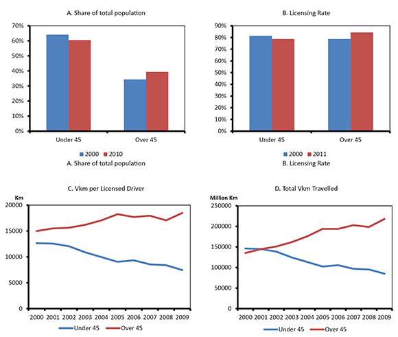
Changing population and demographic trends are expected to have an impact on future economic and energy use trends. This appears to be particularly true for the case of transportation, as was highlighted in the Energy Context section of EF 2013. Using the available Canadian data,[3] Figure 1 illustrates several key trends in population and transportation by comparing driving-age people under 45 as well as 45 and older.
Figure 1: Transportation and Demographic Trends by Age Group
Text version of this graph
This figure illustrates various trends in demographics and driving behaviour in Canada. Figure 1a shows that the share of Canada’s population under 45 years old decreased from 64 per cent in 2000 to 61 per cent in 2001. Figure 1b shows that between 2000 and 2011, the licensing rate, which is the share of a given age group population with a driver’s licence, declined for younger age groups and increased for older age groups. Figure 1c shows that the vehicle kilometres travelled per licensed driver increased for older age groups, but declined for younger age groups, between 2000 and 2009. Figure 1d shows that total vehicle km travelled increased for older age groups, but declined for younger age groups, between 2000 and 2009.
Source: Statistics Canada, Transport Canada, NEB
These charts illustrate several trends in Canadian demographics and transport demand over recent history:
- Older age groups are becoming a larger share of the population.
- The licensing rate, which is the share of a given age group population with a driver’s licence, is declining for younger age groups and increasing for older age groups.
- Of those people that do have a driver’s licence, younger drivers are driving less, while older drivers are driving more.
- As a result, total vehicle km (VKm) travelled by drivers in the younger age group fell over the period, and increased in the older age group.
Overall, total Vkm travelled by personal vehicles increased by approximately 20 billion Km from 2000 to 2009. A statistical method called factorization analysis provides a way to analyse the relative impact of the changing trends shown in Figure 1 on total Vkm travelled. This type of analysis is used by Natural Resources Canada in their Energy Efficiency Trends Analysis work as a way to separate the impact of activity, structural and intensity effects on energy use. Figure 2 applies this technique to VKm and demographic trends.[4] In this case the change in total Vkm travelled relative to 2000 (dashed black line) is broken down into four effects: Population Effect, Demographic Structure Effect, Licensing Rate Effect, and Driving Intensity Effect. The sum of these four effects adds up to the total change in VKm in any given year.
Figure 2: Change in VKm Relative to 2000, Decomposed into Four Effects

Text version of this graph
Figure 2 illustrates the change in total vehicle km travelled in Canada relative to 2000, broken down into various effects that influence travel use. It shows that rising population and an aging demographic structure has an upward impact on vehicle km travelled, changes in the licensing rate had a limited impact, and changes in driving intensity had a downward impact on vehicle km travelled.
- Population Effect: the impact of overall driving-age population growth over the time period. Population increased steadily over this period, so there is an increase of the driving age population which leads to upward pressure on the total VKm travelled.
- Demographic Structure Effect: the impact of the changing age structure of the population. Older age groups increased their share of the population over this period. Since older age groups tended to drive more, the aging of the population leads to further upward pressure on total VKm travelled.
- Licensing Rate Effect: the impact of the changing share of licensed drivers within a given age group. As Figure 2 shows, this impact had a small effect over the period, suggesting the impact of a decreasing licensing rate among younger generations is offset by an increasing licensing rate among older generations.
- Driving Intensity Effect: the impact of changes in how much licensed drivers actually drive. This is the key effect reducing overall driving activity. Although Figure 1 shows that licensed drivers from older age groups drive more over this period, on an aggregate level, the decline in driving activity among younger drivers has a bigger impact.
Figure 2 highlights the importance of demographic trends in driving behavior and the significant impact that reduced driving by younger age groups is having on overall transport activity. There is a growing body of research devoted to unravelling these trends further, although much of it focuses on similar trends in the United States (U.S.)[5] Explanations for these changing patterns are varied and include: the impact of rising costs (including fuel, purchase, maintenance and insurance), changing income and employment trends, socioeconomic and cultural factors, and changing technology.
Sensitivity Analysis
Given this uncertainty, two sensitivity cases are created to explore the potential future impacts of these trends on energy use:
- High VKm Case: trends of increased driving intensity and licensing rates from the older age groups continue, while the decreasing trends from younger age groups flatten and/or reverse.
- Low VKm Case: trends of decreasing driving intensity and licensing rates from the younger age groups continue, while the increasing trends from older age groups flatten and/or reverse.
Table 1 shows the average annual growth rate for VKm in personal vehicles and passenger energy use over the projection period. Energy prices, population trends (including overall growth and demographic structure), and other macroeconomic variables remain at the Reference Case levels.
Table 1: VKm and Energy Use by Case
| VKm in Personal Vehicles, Average Annual Growth, 2012-2035 (per cent) |
Passenger Energy Use, Average Annual Growth, 2012-2035 (per cent) |
|
|---|---|---|
| Reference Case | 1.0 | -1.0 |
| High VKm Case | 1.6 | -0.5 |
| Low VKm Case | 0.5 | -1.5 |
Figure 3 compares Vkm travelled in personal vehicles (dashed lines) and passenger sector[6] energy use (solid lines) in the Reference Case to the High and Low VKm Cases. Passenger energy use, measured in petajoules (PJ) continues to decline in all of the sensitivity cases. This highlights the impact of the efficiency improvement in passenger vehicles that is expected over the projection period.[7] In the High VKm Case, passenger energy use declines at an average annual rate of 0.8 per cent, or approximately 17 per cent over the projection period. In the Low VKm Case, passenger energy use declines by an average of 1.8 per cent per year, nearly 35 per cent over the 2012-2035 projection period.
By 2035, passenger energy use is 13 per cent higher than the Reference Case in the High VKm Case, and 10 per cent lower than the Reference Case in the Low VKm Case, and 10 per cent lower than the Reference Case in the Low VKm Case.
Figure 3: Passenger Energy Use (Excluding Aviation) and VKm Travelled, Reference Case and Sensitivities

Text version of this graph
Figure 3 illustrates passenger energy use (excluding aviation) and vehicle km travelled over the projection period (2012 to 2035) for three cases: the Reference Case, the High VKm Case, and the Low Vkm Case. It shows that even though travel increases in all three cases, energy use declines at varying rates. This is due to the impact of efficiency improvements.
Chapter 2. Long-term Uncertainties in Natural Gas Use
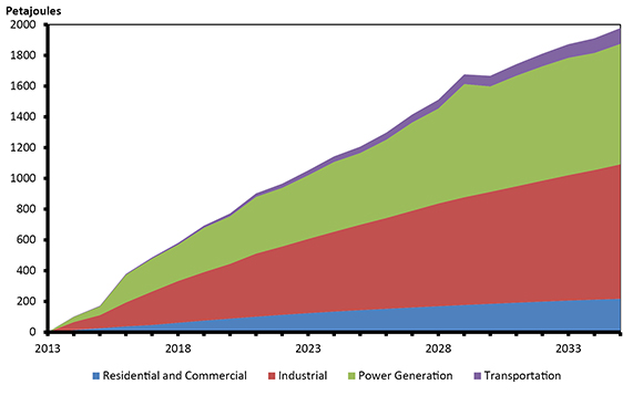
EF 2013 projects natural gas to be the fastest growing fuel in Canadian primary demand over the projection period. Figure 4 shows the growth in natural gas primary demand relative to 2013 by sector. Overall, primary natural gas demand increases by an average annual rate of 1.7 per cent (approximately 1 900 PJ or 5 billion cubic feet per day (Bcf/d)) from 2012 to 2035. The projected growth in natural gas use is dominated by increases in power generation and industrial use. The power generation demand growth is driven by retiring coal units, as well as meeting increasing demands for electricity. Key drivers of the industrial growth include use by natural resource industries, such as oil sands and other energy-intensive industries. The growth in transportation use is notable as well: although it is a fairly small share, the use of natural gas in transportation increases from one PJ in 2012 to over 100 PJ in 2035.
Figure 4: EF 2013 Reference Case Growth in Primary Natural Gas Demand 2012-2035, by Sector
Text version of this graph
Figure 4 illustrates projected growth in natural gas energy use from the EF 2013 Reference Case, 2012 to 2035. In this projection, the largest growth areas for natural gas consumption are the industrial and power generation sectors.
To explore this trend further, additional sensitivity cases are created to analyze the impact of alternative assumptions related to oil sands and power generation natural gas use and the potential for an even greater increase in transportation demand.
2.1 Natural Gas in Transportation
Issue and Background
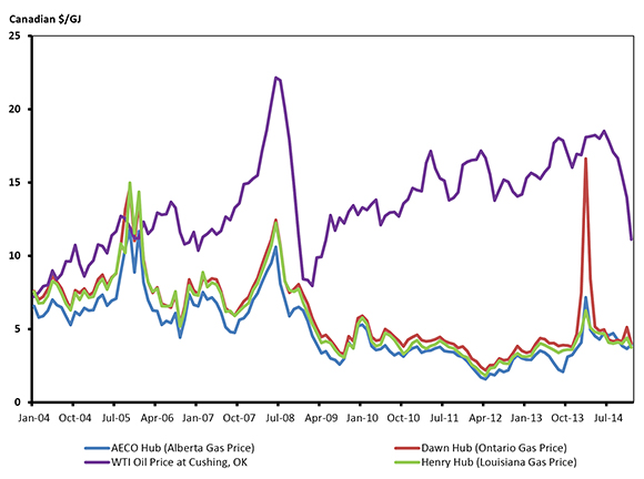
In recent years, there has been interest in capitalizing on the price differential between crude oil and natural gas (Figure 5) by substituting natural gas for oil products. The transportation sector uses the majority of liquid fuels in the U.S. and Canada, representing a target for oil-to-natural gas substitution.
Figure 5: Crude oil and Natural Gas Price on an Energy Equivalent Basis, Monthly, 2004 to 2014
Text version of this graph
Figure 5 compares trends in the price of crude oil (using the WTI oil price at Cushing, OK) and various natural gas price benchmarks: AECO Hub (Alberta), Dawn Hub (Ontario), and Henry Hub (Louisiana). It shows that on an energy equivalent basis, the differential between crude oil and natural gas prices has been much higher in recent years than it was in 2004 and 2005. However, it has narrowed substantially with the recent decline in crude oil price.
Source: GLJ
Much of the interest in natural gas as a transportation fuel is for medium and heavy duty freight trucks. As noted in EF 2013, this interest is primarily in operations where the vehicles return to central locations often and use regional transport corridors. Several fueling stations are in place or are currently being constructed in key strategic highway locations. An emerging area of interest is using natural gas as a fuel for rail freight transport.
There are a variety of additional costs and uncertainties with switching from crude oil to natural gas. The capital cost of incremental natural gas vehicles (NGVs) and locomotives are higher than their diesel counterparts.[8], [9] There are a variety of infrastructure concerns, particularly related to refueling. Also, the persistency of the differential is uncertain and can be volatile, particularly with the recent natural gas price increases in winter 2013 and the recent declines in oil prices (Figure 5).
Sensitivity Analysis
The EF 2013 demand projections included a modest penetration of natural gas in the freight transportation sector. To explore the impact of additional natural gas use for freight transportation, two additional sensitivity cases are created. These sensitivity cases are:
- The High NGV Case: assumes a higher penetration rate of medium and heavy duty natural gas powered freight trucks than in the Reference Case.
- High NGV+Rail Case: penetration of NGV trucks consistent with the High NGV case, combined with a high penetration of natural gas-powered locomotives in rail freight transportation.
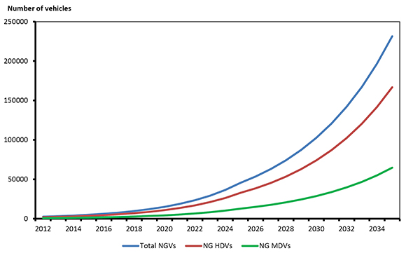
There are two options in using natural gas for vehicles: compressed natural gas (CNG) and liquefied natural gas (LNG). Due to the size constraints imposed on CNG fuel tanks resulting from CNG’s high diesel gallon equivalency (DGE),[10] it is most suited for short-haul applications and is assumed to be adopted only by medium duty vehicles (MDVs). With a lower DGE and a shorter shelf-life,[11] LNG can handle larger amounts of fuel for both long-hauls and other applications that require constant fuel use. LNG is therefore assumed to be adopted by heavy duty vehicles (HDVs) and train locomotives.
In the High NGV Case, NGV adoption targets are created based on the Energy Information Administration’s (EIA) 2012 Issues in Focus section of its Annual Energy Outlook (AEO) and other external reports.[12] The number of medium and heavy NGVs in the High NGV Case are shown in Figure 6. The number of NGVs in the High NGV Case increases to over 200 000 vehicles by 2035, while the Reference Case projection was consistent with 50 000 to 60 000 MDVs and HDVs.
Figure 6: Freight NGV Projection in the High NGV Case
Text version of this graph
Figure 6 illustrates the number of freight medium and heavy duty natural gas vehicles that are assumed in the High NGV Case. The total number of NGVs in the High NGV Caseincreases to over 200 000 vehicles by 2035, with a higher number of heavy duty vehicles compared to medium duty.
Locomotive adoption targets are based upon the ‘High Rail LNG’ Case from the EIA’s projection in the Issues in Focus section of the AEO 2014. This Case involves a transformative change in the rail industry, where natural gas meets 95 per cent of freight rail energy demands by 2040 (approximately 90 per cent in 2030).
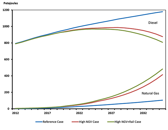
Figure 7 illustrates the impact that freight NGV adoption had on total freight, diesel and natural gas demand over the projection. By 2035, natural gas usage is over 300 PJ higher than its Reference Case level, while diesel use is 287 PJ lower.[13]
Figure 7: Freight Diesel and Natural Gas Demand by Case
Text version of this graph
Figure 7 illustrates projected natural gas and diesel use in three cases: the Reference Case, the High NGV Case, and the High NGV+Rail Case. By 2035, natural gas use is 300 petajoules higher in the High NGV case compared to the Reference Case, while diesel is 287 petajoules lower.
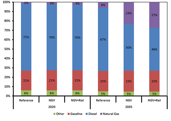
Figure 8 illustrates how the freight transportation (excluding air) fuel mix changes between the cases in 2020 and 2035. In 2020, the difference between the cases is limited, with the share of natural gas in the NGV+Rail Case approximately one per cent higher than in the Reference Case. This limited medium term impact illustrates the gradual nature of adopting a new technology. By 2035 the impact is larger: natural gas accounts for 23 per cent of freight demand in the NGV Case, and 27 per cent in the NGV+Rail Case, relative to just six per cent in the Reference Case. The share of diesel drops to 50 per cent in the NGV Case and 46 per cent in the NGV+Rail Case.
Figure 8: Share of Fuel Use in Freight Transportation by Case, 2020 and 2035
Text version of this graph
Figure 8 illustrates the share of fuel use in freight transportation in 2020 and 2035 across three cases: the Reference Case, the High NGV Case, and the High NGV+Rail Case. It shows that the penetration of natural gas vehicles is fairly low in all three cases in 2020. By 2035, natural gas accounts for 23 per cent of freight demand in the High NGV Case, and 27 per cent in the High NGV+Rail Case, compared to six per cent in the Reference Case.
2.2 Natural Gas Intensity for Oil Sands
Issue and Background
In EF 2013, natural gas use by the oil sands is one of the key growth areas for overall energy use. Purchased natural gas requirements for the oil sands (including cogeneration) rise to 95.1 106m³/d (3.4 Bcf/d) by 2035. Much of this growth is from in situ production, which EF 2013 projects to be the largest source of oil production growth over the projection period. The thermal in situ process is energy intensive, involving injecting steam into the ground to heat up the bitumen in the oil reservoir, reducing its viscosity enough to be pumped to the surface.
In situ’s Steam Oil Ratio (SOR) is the ratio of the volume of steam required to produce the same volume of oil. Higher SORs are the result of more steam being used to produce a barrel of oil. Since natural gas is used to create the steam, the SOR is a measure of natural gas intensity.
There are a variety of ways to measure SOR:
- Instantaneous SOR (iSOR): iSORs are loosely defined as the SOR of a facility or reservoir at a given moment in time, which is typically measured from monthly production. iSORs are higher at initial production stages as more energy is needed to overcome some production inertia. When production becomes consistent, iSORs decline, with the rate of decline plateauing after several years. Maturing reservoirs may start to exhibit a modest iSOR increase as more effort is needed to keep up current production rates.
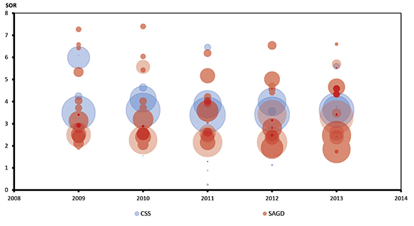
- Annual SORs at Project Level: ratio of a project’s annual steam usage to annual bitumen production. This measure provides a useful way of comparing the annual efficiency performance of various sites across time. Figure 9 displays annual SORs for various Cyclic Steam Stimulation (CSS) and Steam Assisted Gravity Drainage (SAGD) projects from 2009 to 2013[14] and illustrates the variation that exists between them. The points are scaled by the facilities’ production levels, with larger circles representing higher production. Figure 9 illustrates that extreme outliers in terms of SOR (both high and low) often are producing at low levels.
Figure 9: Annual SORs at Project Level, 2009-2013
Text version of this graph
Figure 9 illustrates annual SORs at project level from 2009 to 2013. For each year there are a number of circles representing individual facilities, where the size is scaled to the facility’s oil production number. It shows a high level of diversity in SORs at project level, with extreme outliers (both high and low) producing at low levels. Generally, the majority of SAGD facilities have a lower SOR than CSS facilities.
Source: AER
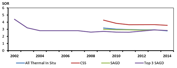
- Aggregate Production-Weighted SOR: ratio of the annual steam usage to annual bitumen production for the entire industry or production type. This measure is useful to compare recovery processes or measure the efficiency of in situ in general. Figure 10 presents the aggregate production-weighted SOR for CSS, SAGD and thermal in situ and shows that CSS production has a consistently higher production-weighted SOR than SAGD. Figure 9 highlights this as well, as the blue circles have most of their area located above the area of the red circles. This high-level efficiency measure provides the basis for long-term energy modeling analysis.
Figure 10: Historical aggregate production-weighted SOR - In Situ Projects
Text version of this graph
Figure 10 illustrates historical aggregate production-weighted SOR values. It shows the aggregate production weighted SOR for the top 3 SAGD facilities from 2002 to 2014. From 2009 to 2014, aggregate data for CSS, SAGD and total in situ facilities are shown. The figure shows that SAGD SOR levels declined significantly from 2002 to 2014, and that CSS production has a consistently higher production-weighted SOR than SAGD.
* Top Three SAGD producers are Foster Creek, Firebag and Mackay River, which represented a large majority of production from 2002-2008 and therefore offer a good measure of in Situ's aggregate production-weighted SOR over that period.
Source: Alberta Energy and AER
Despite the fact that in situ’s SOR has declined since the inception of SAGD in 2002, the recent flat-line in Figure 10, as well as the volatility shown in Figure 9, is indicative of the current uncertainty regarding where energy intensity is heading. While the distribution of CSS SOR data has exhibited fairly consistent SORs over the five year period, SAGD has seen variation persist around the SOR level of three, so it is unclear where the overall values are trending.
Adding to the future uncertainty is that these charts only account for existing facilities. Much of the incremental production over the EF 2013 projection period will involve exploiting new reservoir types with methods which have unknown natural gas intensities. Recent projects have encountered increasing levels of heterogeneity[15] in the reservoir rock. This has increased the steam requirements for many facilities and in turn, spurred the continuing pursuit of innovative solutions to enhance SAGD recovery and reduce the SOR. Examples of such innovations include injecting methane or solvent with steam, and drilling vertical infill wells between SAGD wells in an attempt to recover bitumen from outside of the reservoirs that have been mobilized by heat escaping from them. These, along with several other innovative processes, are currently being implemented or are in the testing phase. Work is also being done to identify an economic means of exploiting the bitumen locked in the Grosmont carbonates, with the most notable method being electromagnetic-assisted SAGD, where electrodes are inserted into wells that can target the bitumen for heating with electromagnetic radiation.
Key questions for the future include:
- Will process improvements be enough to counter the challenges of heterogeneous reservoirs?
- Given these process improvements and heterogeneous reservoirs, what will the new facility-level SORs be and to what degree will they alter in situ’s aggregate production-weighted SOR?
- With in situ providing over 70 per cent of the incremental production over the EF forecast, and significant variations in SORs possible from year-to-year for a given well, what effect will a distribution of new and aging existing reservoirs have on aggregate production-weighted SORs in a given year of the projection?
Sensitivity Analysis
The EF 2013 Reference Case assumes a 0.5 per cent decrease in the SOR over the forecast period. But future efficiencies may be higher or lower, depending on the answers to the above questions. Because of the uncertainty in natural gas efficiency and the fact that in situ production is expected to be such an integral component of the projection’s natural gas demand, it is worth exploring how natural gas use would change under alternative SOR assumptions.
To explore the uncertainty around in situ natural gas use and efficiency, three alternative sensitivity cases are created and compared to the Reference Case. These are:
- High SOR Case: one per cent annual increase in SOR over projection
- Constant SOR Case: constant SOR over projection
- Low SOR Case: two per cent annual decrease in SOR over projection
Figure 11 illustrates how these assumptions affect the SORs over the forecast period. Although these cases vary widely, the range of the aggregate SOR values shown in Figure 11 are within the majority of facility production-weighted SOR values shown in Figure 9. It is important to note that this analysis assumes that oil sands production growth is equal to the Reference Case in the sensitivity cases. This may not hold. Higher or lower SOR values, implying higher or lower productivity and/or natural gas requirements by project, may alter project economics and impact production growth and therefore affect total oil sands natural gas requirements. This analysis ignores these dynamics in an effort to illustrate how sensitive both the oil sand requirements and the total Canadian demand for natural gas are to SOR assumptions in the EF 2013 projection.
Figure 11: 2035 SOR Assumptions, Reference and Sensitivity Cases
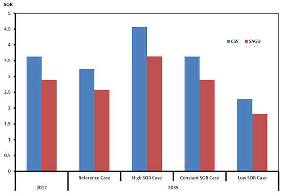
Text version of this graph
Figure 11 shows the CSS and SAGD SOR values in 2035 for the Reference Case and alternative cases. In the Reference Case, the SOR values decline by 0.5 per cent per year. In the Constant SOR Case, the values are equivalent to 2012 levels. In the High SOR Case, the values increase by one per cent per year. In the Low SOR Case, the values decline by two per cent per year.
Figure 12 illustrates how sensitive total oil sands natural gas purchase requirements[16] are to changes in the SOR. Oil sands natural gas purchase requirements range 51.4 106m³/d (1.81 Bcf/d) between the High and Low SOR Cases in 2035. In 2035, natural gas use in the High SOR Case is 29.9 106m³/d (1.06 Bcf/d) over the Reference Case, and 21.5 106m³/d (0.76 Bcf/d) under the Reference Case in the Low SOR Case.
Altering the SOR assumptions has a notable impact on total Canadian natural gas demand. In the Reference Case, total primary natural gas demand increases at an average annual rate of 1.7 per cent, approximately 140 106m³/d (5 Bcf/d; as shown in Figure 4). In the High SOR Case, primary natural gas demand increases by over 170 106m³/d (6 Bcf/d) over the projection period, an average annual growth of two per cent per year. In the Low SOR Case, primary natural gas demand growth is 120 106m³/d (4.2 Bcf/d), an average annual growth of 1.5 per cent per year. In 2035, total Canadian natural gas demand is eight per cent below the Reference Case in the Low SOR Case and six per cent above the Reference Case in the High SOR Case.
Figure 12: Purchased Natural Gas for Oil Sands Extraction and Upgrading, by Case

Text version of this graph
Figure 12 illustrates purchased natural gas for oil sands extraction and upgrading over the projection period for the Reference Case, Constant SOR Case, Low SOR Case, and High SOR Case. It shows that oil sands natural gas requirements are sensitive to SOR. Oil sands natural gas purchase requirements range 51.4 million cubic metres per day(1.81 billion cubic feet per day) between the High and Low SOR cases in 2035.
2.3 Carbon Capture and Storage (CCS) and Natural Gas Combined Cycle Power Generation
Issue and Background
As noted in EF 2013, federal regulations enacted in 2012 require new coal plants to reduce GHG emissions to no more than 420 metric tons of carbon dioxide (CO2) per gigawatt hour (GWh). The regulation outlines stringent performance standards for new coal-fired electricity generation units and units that have reached the end of their useful life. Effectively, any new coal facility built after July 2015 is equipped with CCS. In EF 2013, several CCS facilities in Alberta and Saskatchewan come online over the projection period, reaching nearly 2 000 MW of capacity in 2035. Much of the growth in CCS occurs after 2020, replacing retired coal units or as a retrofit to existing coal plants.
Both Alberta and Saskatchewan are endowed with rich coal resources and are pursuing CCS technology to take advantage of the abundant resource and to satisfy future electricity demand. In the past few years, Alberta and Saskatchewan have announced long-term strategies, projects and financial commitments to assist in the building of coal power plants with CCS technology. The $1.35 billion Boundary Dam CCS project in Saskatchewan opened in 2014. It is the world’s first and largest commercial-scale CCS project, and is capable of producing 110 MW.
CCS is an emerging technology, and its long-term growth is uncertain. In the EF 2013 Reference Case, natural gas-fired generation supplies the majority of future electricity requirements in the two provinces. The EIA estimates of capital costs and energy requirements for natural gas combined cycle (NGCC) and CCS plants (Table 2) show lower costs for NGCC on a per kW basis. The Alberta Electric System Operator’s (AESO) 2014 Long Term Outlook anticipates no new coal-fired plants over the next 20 years, mainly because of the unfavorable economics of CCS. Instead, the AESO Outlook anticipates combined cycle natural gas-fired generation to replace retiring coal-fired generation.
Table 2: Capital Cost Estimates for Utility Scale Electricity Generating Plants
| Nominal Capacity (MW) |
Heat Rate (Btu/kWh) |
Overnight Capital Cost[17] ($/kW) |
Fixed O&M Cost ($/kW-yr) |
Variable O&M Cost ($/MWh) |
|
|---|---|---|---|---|---|
| Coal Single Unit Advanced PC with CCS | 650 | 12 000 | 5 227 | 80.53 | 9.51 |
| Coal Dual Unit Advanced PC with CCS | 1 300 | 12 000 | 4 724 | 66.43 | 9.51 |
| Natural Gas Conventional CC | 620 | 7 050 | 917 | 13.17 | 3.60 |
| Natural Gas Advanced CC | 400 | 6 430 | 1 023 | 15.37 | 3.27 |
| Natural Gas Advanced CC with CCS | 340 | 7 525 | 2 095 | 31.79 | 6.78 |
Source: EIA[18]
Sensitivity Analysis
Considering these uncertainties, it is interesting to ask what the electricity and energy use impacts would be if the EF 2013 CCS additions are replaced with natural gas. The Capacity Switch Case assumes that the long-term CCS capacity additions included in the Reference Case are removed and replaced with NGCC units with the same generating capacity.
Figure 13 compares Canada’s capacity mix in 2035 for the Reference and Capacity Switch Cases. Relative to the Reference Case, the share of natural gas increases in the Capacity Switch Case, and the share of coal declines. EF 2013 projects Canada’s total installed capacity to be over 164 000 MW by 2035, so the shift of 2 000 MW from coal to natural gas changes capacity shares by one per cent. This has the largest impact on coal use. The Capacity Switch Case shows that without the long-term CCS additions, projected coal capacity is lower than some renewable sources (non-hydro, non-wind[19]) while in the Reference Case the shares were about the same.
Figure 13: Canadian Capacity Mix in 2035, Reference and Capacity Switch Case

Text version of this graph
Figure 13 illustrates the projected Canadian electric capacity mix in 2035 for the Reference Case and the Capacity Switch Case. It shows that without the CCS additions assumed in the Reference Case, natural gas capacity is higher in the Capacity Switch Case (23 per cent, compared to 22 per cent in the Reference Case) while coal and coke capacity is lower (three per cent, compared to four per cent in the Reference Case).
Figure 14 shows the share of natural gas-fired generation for Alberta and Saskatchewan in 2035 for the Reference and Capacity Switch Cases. The Reference Case values reflect strong growth in natural gas generation, with natural gas reaching 68 per cent of the 2035 generation mix in Alberta, and 59 per cent in Saskatchewan.[20] In the Capacity Switch Cases, the reliance on natural gas generation is even higher. In Alberta, natural gas powers three quarters of the 2035 generation in the Capacity Switch Case, while in Saskatchewan natural gas makes up nearly 65 per cent of the generation mix.
Figure 14: Share of Natural Gas-fired generation, Alberta and Saskatchewan in 2035, Reference and Capacity Switch Case
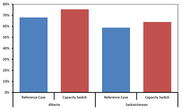
Text version of this graph
Figure 14 compares the share of natural gas-fired generation in 2035 between the Reference Case and the Capacity Switch Case for Alberta and Saskatchewan. It shows that in the Capacity Switch Case, the share of natural gas-fired generation in Alberta increases to 75 per cent in the Capacity Switch Case, while in Saskatchewan it increases to 65 per cent.
This shift also has implications for primary energy demand, as shown in Table 3. In the Capacity Switch Case, Canadian coal demand for power generation is 34 per cent or 130 PJ (5.5 Megatonnes) lower than the Reference Case in 2035. Natural gas demand for power generation becomes an even stronger driver for overall natural gas use. Canadian primary natural gas demand for power generation in the Capacity Switch Case is six per cent higher than the Reference Case in 2035 (approximately 75 PJ[21] or 0.2 Bcf/d), growing to 1 450 PJ (approximately 4 Bcf/d).
Table 3: Power Generation Demand by Case, 2035
| Reference Case (PJ) | Capacity Switch Case (PJ) | Per Cent Change | |
|---|---|---|---|
| Natural Gas | 1 374 | 1 450 | 6% |
| Coal | 387 | 257 | -34% |
Chapter 3. Powering LNG: Alternative options
Issue and Background
The future for LNG exports is a key uncertainty in Canada’s energy system. Currently there are a large number of proposed LNG export projects in British Columbia (B.C.) and a smaller number proposed on the East Coast. As of December 2014, none of the export project proponents have announced final investment decisions. To deal with this uncertainty, EF 2013 assumed one Bcf/d of LNG exports in 2019, two Bcf/d in 2021 and three Bcf/d by 2023.
When it comes to future energy use, an important uncertainty of potential LNG exports is the energy required to power the LNG export facilities. According to BC Hydro, LNG-related electricity demand falls into two general categories: compression (liquefying natural gas) and non-compression. Energy demand for compression is approximately 85 per cent[22] of the total plant’s energy needs. The remaining (non-compression) energy requirement is for plant pumps, motors, other equipment, heating and lighting.
EF 2013 assumes that all energy use related to LNG export facilities comes from natural gas-fired electricity plants. An additional 450 MW combined cycle unit is added in each of the years 2019, 2021, and 2023, corresponding to each assumed increment of LNG exports. At an end-use level, the electricity used by these plants was included in the industrial energy demand projection for B.C.
EF 2013 also noted this was only one of several potential options for meeting this demand. New LNG export facilities have a number of options to power their facilities. These options include:
- Direct Drive: uses natural gas as a fuel source to turn gas turbines for the liquefaction process. In most LNG plants, compression requirements are typically supplied with direct drive.
- Electric Drive, Self-generation: uses large electric motors to drive the compressors. Power is generated on-site by the LNG producer using natural gas as fuel source.
- Electric Drive, Grid Purchases: uses large electric motors to drive the compressors. Power is purchased directly from the B.C. grid.
BC Hydro projects LNG non-compression demand could be one of the biggest system loads, adding an additional peak demand ranging between 100 to 800 MW. Compression demands are expected to be met with direct drive or self-generation.
LNG project descriptions that were submitted to the Canadian Environmental Assessment Agency (CEAA)[23] and various project websites[24] shed some light as to how some of the proposed LNG projects plan to power their facilities. These are included in Table 3, and often involve some combination of the various options.
The Woodfibre LNG project is planning to purchase power directly from the grid as they try to take advantage of existing infrastructure that is already in place. The Pacific Northwest LNG project plans to generate its own power for the compression process while considering grid purchase for the non-compression demand. The LNG Canada project description states their intention to use natural gas direct drive for the compression process while considering purchasing power from the grid for auxiliary power. Recently LNG Canada has announced[25] that, if their project proceeds, they will be using GE’s aeroderivative gas turbine for the compression process and power purchased form BC Hydro for the non-compression process. The Prince Rupert LNG project plans to design a self-sufficient facility where it has the capability to meet its entire power requirement.
Table 4: Proposed Canadian LNG Export Projects That Have Stated Their Facility Powering Options
| Project Description | Facility powering option | Estimated Load (MW) | |||||
|---|---|---|---|---|---|---|---|
| Name | Proponents | Location | Bcf/d | Compression | Non-compression | Non-compression | Total |
[*] Highest load expected at full operation [**] Highest load expected at full operation (at completion of phase 1) |
|||||||
| LNG Canada | Shell Canada, PetroChina, Korea Gas & Mitsubishi | Kitimat | 3.71 | Direct drive | Grid Purchase | 150 | 150 |
| Pacific Northwest LNG | PETRONAS, JAPEX | Prince Rupert | 3.15 | Direct drive/Self-generation | Self-generation/ Other | 380 | 700[*] |
| Prince Rupert LNG | BG Group | Prince Rupert | 3.34 | Direct drive | Self-generation/Grid Purchase | 200 | 800 |
| Woodfibre LNG | Pacific Oil and Gas Group | Squamish | 0.33 | Grid Purchase | Grid Purchase | unknown | 140 |
| Aurora | Nexen, INPEX, JGC | Prince Rupert | 3.11 | Direct drive | Self-generation | unknown | 300[**] |
Source: CEAA, Project Websites
Sensitivity Analysis
To analyze the impact of alternative methods of powering LNG on B.C. energy use, two alternative sensitivity cases are developed and compared with the Reference Case. These cases maintain the EF 2013 assumptions of one Bcf/d of LNG export in 2019, two Bcf/d in 2021 and three Bcf/d in 2023 (where it remains for the rest of the projection period), which are not related to any specific project.
The cases are described in Table 5. The alternative cases both assume that compression demands (85 per cent of total) are met by direct drive. This is in contrast to the Reference Case, where compression demands are met through electric drive. The alternative cases differ in how they treat non-compression demands. The Direct Drive/Self-generation Case assumes non-compression demands are met by self-generation via NGCC. The Direct Drive/Grid Purchase Case assumes that the non-compression requirement is met with electricity purchased from the grid.
Table 5: Powering LNG: Alternative Options Case Description
| Case | Description |
|---|---|
| Reference Case (Electric Drive) |
Total LNG demands met by using 0.2 Bcf/d of natural gas to generate 10 567 GWh of electricity for compression (electric drive) and non-compression demands |
| Direct Drive/ Self-generation |
Compression demands: Met by using 0.17 Bcf/d of natural gas directly Non-compression demands: Met by using 0.03 Bcf/d of natural gas to generate 1 528 GWh of electricity |
| Direct Drive/ Grid Purchases |
Compression demands: Met by using 0.17 Bcf/d of natural gas directly Non-compression demands: No additional capacity assumed to meet the 1 528 GWh of electricity. This demand is purchased from the grid. |
Figure 15 shows B.C.’s total primary natural gas use in 2035 for the three cases, disaggregated by sector. Overall, the difference between these cases is fairly nuanced. As the figure shows, overall primary natural gas demand does not change much between the Reference Case and the Direct Drive/Self-generation Case.[26] However, the sector using the energy for compression does change, as the energy used to generate natural gas in the Reference Case is now used directly in the industrial sector by the LNG facilities. Non-compression demands are satisfied through natural gas-fired generation, as in the Reference Case.
Figure 15: B.C. Natural Gas Demand by Sector, 2035
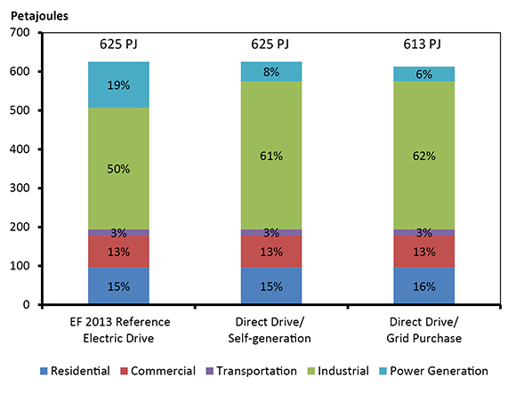
Text version of this graph
Figure 15 compares B.C. natural gas demand by sector in 2035 across the Reference Case, Direct Drive/Self-generation Case, and Direct Drive/Grid Purchase Case. It shows a higher percentage of natural gas used directly in the industrial sector for the alternative cases compared to the Reference Case. Also, the total natural gas used in the Direct Drive/Grid Purchase sector is 613 petajoules, compared to 625 petajoules in the other cases.
The Direct Drive/Grid Purchase Case is identical to the Direct Drive/Self-generation Case for compression demands. The difference occurs on the non-compression side. In the Self-generation Case, approximately 200 MW of natural gas-fired capacity is added to satisfy this demand directly. In the Grid Purchase Case this capacity is not added, and the electricity demands (1 500 GWh by 2035) are met with electricity purchased from the grid. In this analysis, all other assumptions are constant at Reference Case levels, and so these incremental electricity requirements are met mostly through reduced net exports. However, other possibilities include adding additional capacity (such as renewables), or taking additional demand-saving actions.
Summary of Results
| Topic | Sensitivity Case | Description | Results |
|---|---|---|---|
| 1.0 Transport Demand and Demographic Trends | High VKm Case | Trends of increased driving intensity and licensing rates from the older age groups continue, while the decreasing trends from younger age groups flatten and/or reverse. |
|
| Low Vkm Case | Trends of decreasing driving intensity and licensing rates from the younger age groups continue, while the increasing trends from older age groups flatten and/or reverse. |
|
|
| 2.1 Natural Gas in Transportation | High NGV Case | Assumes a higher penetration rate of medium and heavy duty natural gas powered freight trucks (over 200 000 by 2035) than in the Reference Case (approximately 50-60 000 by 2035) |
|
| High NGV+Rail Case | Natural gas-fueled freight trucks, plus a high penetration of natural gas in freight rail transportation. |
|
|
| 2.2 Natural Gas Intensity for Oil Sands | High SOR Case | In situ oil sands SOR is assumed to increase at an average of one per cent per year over the projection period. In the Reference Case, it is assumed to decline by 0.5 per cent per year. |
|
| Constant SOR Case | In situ oil sands SOR is assumed to remain constant over the projection period. |
|
|
| Low SOR Case | In situ oil sands SOR is assumed to decrease at an average of two per cent per year over the projection period. |
|
|
| 2.3 CCS and Natural Gas Combined Cycle Power Generation | Capacity Switch Case | Long-term Reference Case CCS capacity additions in Alberta and Saskatchewan (approximately 2 000 MW) are replaced with natural gas combined cycle. |
|
| 3. Powering LNG: Alternative Options | Direct Drive + Self- generation Case | LNG compression requirements (approximately 85 per cent of facility energy requirements) are met by “direct drive” technology, where natural gas is used directly. Non-compression requirements (the other 15 per cent of facility energy requirements) are met through on-site natural gas-fired generation. The Reference Case assumes all LNG requirements were met through natural gas-fired generation. |
|
| Direct Drive + Grid Purchase Case | LNG compression requirements are met by direct drive, which reduces the gas-fired capacity relative to the Reference Case. Non-compression requirements are met through grid purchases. |
|
About this Report
The National Energy Board (NEB or Board) is an independent federal regulator whose purpose is to promote safety and security, environmental protection and efficient infrastructure and markets in the Canadian public interest within the mandate set by Parliament for the regulation of pipelines, energy development, and trade.
The Board's main responsibilities include regulating:
- the construction, operation and abandonment of oil and gas pipelines that cross international borders or provincial/territorial boundaries, as well as the associated pipeline tolls and tariffs;
- the construction and operation of international power lines, and designated interprovincial power lines; and
- imports of natural gas and exports of crude oil, natural gas, oil, natural gas liquids (NGLs), refined petroleum products and electricity.
Additionally, the Board has regulatory responsibilities for oil and gas exploration and production activities in frontier lands not otherwise regulated under joint federal/provincial accords. These regulatory responsibilities are set out in the Canada Oil and Gas Operations Act (COGO Act), the Canada Petroleum Resources Act (CPR Act). For oil and natural gas exports, the Board’s role is to evaluate whether the oil and natural gas proposed to be exported is surplus to reasonably foreseeable Canadian requirements, having regard to the trends in the discovery of oil or gas in Canada. The Board monitors energy markets, and assesses Canadian energy requirements and trends in discovery of oil and natural gas to support its responsibilities under Part VI of the National Energy Board Act (the NEB Act). The Board periodically publishes assessments of Canadian energy supply, demand and markets in support of its ongoing market monitoring. These assessments address various aspects of energy markets in Canada. Canada’s Energy Future 2013: Energy Supply and Demand Projections to 2035 is one such assessment that projects Canadian energy supply and demand trends out to 2035. This report, Energy Futures Supplement: Demand Sensitivities complements the Energy Futures projections by exploring additional areas of long-term interest for Canada’s energy system related to energy use.
If a party wishes to rely on material from this report in any regulatory proceeding before the NEB, it may submit the material, just as it may submit any public document. Under these circumstances, the submitting party in effect adopts the material and that party could be required to answer questions pertaining to the material. This report does not provide an indication about whether any application will be approved or not. The Board will decide on specific applications based on the material in evidence before it at that time.
List of Figures
- 1. Transportation and Demographic Trends by Age Group
- 2. Change in VKm Relative to 2000, Decomposed
- 3. Passenger Energy Use and VKm Travelled, Reference Case and Sensitivities
- 4. EF 2013 Reference Case Growth in Primary Natural Gas Demand 2012-2035, by Sector
- 5. Crude oil and Natural Gas Price on an Energy Equivalent Basis, 2004 to 2014
- 6. Freight NGV Projection in the High NGV Case
- 7. Freight Diesel and Natural Gas Demand by Case
- 8. Share of Fuel Use in Freight Transportation by Case, 2020 and 2035
- 9. Annual SORs at Project Level, 2009-2013 13
- 10. Historical Aggregate Production-Weighted SOR - In Situ Projects
- 11. 2035 SOR Assumptions, Reference and Sensitivity Cases
- 12. Purchased Natural Gas for Oil Sands Extraction and Upgrading, by Case
- 13. Canadian Capacity Mix in 2035, Reference and Capacity Switch Case
- 14. Share of Natural Gas-Fired Generation, Alberta and Saskatchewan in 2035, Reference and Capacity Switch Case
- 15. B.C. Natural Gas Demand by Sector, 2035
List of Tables
- 1. VKm and Energy Use by Case
- 2. Capital Cost Estimates for Utility Scale Electricity Generating Plants
- 3. Power Generation Demand by Case, 2035
- 4. Proposed Canadian LNG Export Projects That Have Stated Their Facility Powering Options
- 5. Powering LNG: Alternative Options Case Description
References, Data Sources, and Further Information
Demographics and Transport Demand
Statistics Canada, Canadian Vehicle Survey. Table 405-0070.
Transport Canada, Canadian Motor Vehicle Traffic Collision Statistics.
Natural Resources Canada, Office of Energy Efficiency. Energy Efficiency Trends Analysis Tables.
EIA, “Light-duty vehicle energy demand: demographics and travel behavior.” Annual Energy Outlook 2014 - Issues in Focus, 2014.
McGuckin, Nancy. “Emerging Trends in U.S. Vehicle Travel Demand.” 2014 EIA Energy Conference Presentations.
Pickrell, Don. “Has Driving Come to a Halt?” 2014 EIA Energy Conference Presentations.
Hutchins, Trisha. “Light-Duty Vehicle Energy Demand, Demographics, and Travel Behaviour.” 2014 EIA Energy Conference Presentations.
Sivak, Michael. “Has Motorization in the U.S. Peaked?” University of Michigan Transportation Research Institute, Report No. UMTRI-2013-17
Schoettle, Brandon and Michael Sivak. “The reasons for the recent decline in young driver licensing in the U.S.” University of Michigan Transportation Research Institute, Report No. UMTRI-2013-22.
Sivak, Michael and Brandon Schoettle. “Recent Changes in the Age Composition of Drivers in 15 Countries.” Traffic Injury Prevention. Volume 13, Issue 2, 2012.
Natural Gas in Transportation
CERI, “Heavy-Duty Diesel Vehicles: Their Carbon-Constrained Future Role within the North American Economy.” Study No. 134, 2013-05.
EIA, “Potential for liquefied natural gas use as a railroad fuel”, EIA: Annual Energy Outlook 2014: Issues in Focus, 2014-04-14. Report number: DOE/EIA-0383(2014).
EIA, “Heavy-Duty Natural Gas Vehicles.” Annual Energy Outlook 2012 - Issues in Focus, 2012.
Fuel Space, “Natural Gas Vehicles in Construction & aggregate Fleets: What You Need to Know.” 2014-11-18.
GLJ Energy Publications, Intra-AB, Dawn and Henry Hub natural gas prices and WTI prices at Cushing, Oklahoma.
Marbek, “Study of Opportunities for Natural Gas in the Transportation Sector.”2010-03.
CN, “CN tests natural gas/diesel fuel powered locomotives between Edmonton and Fort McMurray, Alta.” 2012-09-27.
NRCan, Daily Average Wholesale (Rack) Prices for Diesel.
Smith, Kevin, “LNG: Fuel of the future?” International Railway Journal.
Work Truck Magazine, “Switching to Natural Gas in Medium-Duty Trucks.” 2014-05.
Natural Gas Intensity for Oil Sands
Alberta Energy, “Oil Sands Production Profile.” 2012-04-04.
AER, “ST-53: Alberta Crude Bitumen In Situ Production”. From: 01-2009 to 2014-06.
Gates, I.D & Larter, S.R., “Energy Efficiency and emissions intensity of SAGD.”Fuel, 2013-08-09.
In Situ Oil Sands SOR Reduction Initiative. 2013. Various presentations available.
Carbon Capture and Storage (CCS) and Natural Gas Combined Cycle Power Generation
Alberta Electric System Operator (AESO), “AESO 2014 Long-term Outlook”.
Environment Canada, “Coal-Fired Electricity Generation Regulation-Overview.”
Project Pioneer.
Saskpower, “Carbon Capture Project.”
U.S. Energy Information Administration, “Capital Cost For Electricity Plants.”
Powering LNG Liquefaction Plants
BC Hydro, “Integrated Resource Plan.”
Canadian Environmental Assessment Agency, Project Websites.
Woodfibre LNG project website.
Additional Background Information
Canada’s Energy Future 2013 - Energy Supply and Demand Projections to 2035. Released November 2013.
The 2007, 2009, and 2011 Energy Futures reports are archived.
For background and methodology on the Energy Futures projections, see Energy Futures Backgrounder: Addendum to Canada’s Energy Future: Supply and Demand Projections to 2035. Released June 2012.
List of Acronyms and Abbreviations
| AEO | Annual Energy Outlook |
| AESO | Alberta electric system operator |
| B.C. | British Columbia |
| Bcf/d | Billion cubic feet per day |
| Btu | British thermal unit |
| CCS | Carbon Capture and Storage |
| CEAA | Canadian Environmental Assessment Agency |
| CNG | Compressed natural gas |
| CO2 | Carbon dioxide |
| CSS | Cyclic steam stimulation |
| DGE | Diesel gallon equivalency |
| EF 2013 | Canada’s Energy Future 2013: Energy Supply and Demand Projections to 2035 |
| EFS | Energy Futures Supplement |
| EIA | Energy Information Administration |
| GWh | Gigawatt hour |
| HDVs | Heavy duty vehicles |
| iSOR | Instantaneous Steam oil ratio |
| kWh | Kilowatt hour |
| LNG | Liquefied Natural Gas |
| MDVs | Medium duty vehicles |
| MW | Megawatt |
| MWh | Megawatt hour |
| NEB | National Energy Board |
| NGCC | Natural gas combined cycle |
| NGVs | Natural gas vehicles |
| PJ | Petajoules |
| SAGD | Steam assisted gravity drainage |
| SOR | Steam oil ratio |
| U.S. | United States |
| VKm | Vehicle kilometres travelled |
Endnotes
[1] The most recent Energy Futures outlook is Canada’s Energy Future 2013: Energy Supply and Demand Projections to 2035 (EF 2013) which was released November 2013.
[2] More specifically, scenarios, such as those featured in the 2007 Energy Futures report, are self-contained stories about how the future could unfold. In a scenario, all the key assumptions are subject to change. Sensitivity analysis, featured in this and all subsequent Energy Futures reports, explore how energy outcomes could change based on changes in key assumptions. The impact of changing these assumptions is measured by their difference from the Reference Case.
[3] Vehicle travel data by age group comes from Statistics Canada’s Canadian Vehicle Survey, which was published between 2000 and 2009 (CANSIM table 405-0070). Since the Canadian Vehicle Survey data is estimated based on a sample population, each data point has an associated coefficient of variation which can be used to assess data quality and inferences made based on that data. Data on the number of licensed drivers comes from Transport Canada’s document Canadian Motor Vehicle Traffic Collision Statistics, the latest edition available is for the year 2012.
[4] Specifically, the decomposition methodology is Log-Mean Divisia Index I (LMDI I). The Natural Resources Canada methodology is described in the report prepared by M. K. Jaccard and Associates for the Office of Energy Efficiency, Improvement of the OEE/DPAD Decomposition Methodology, 2005. This report is available by request from the Office of Energy Efficiency. Also see B.W. Ang, A Simple Guide to LMDI Decomposition Analysis.
[5] See, for example, slides from a session devoted to the topic at the 2014 EIA Conference and the Issues in Focus on the topic from the Energy Information Administration’s (EIA) 2014 Annual Energy Outlook (AEO), and recent research from the University of Michigan Transportation Research Institute.
[6] Excludes aviation fuel use.
[7] Efficiency improvements in the three cases are approximately the same, with litres per 100 Vkm declining nearly 40 per cent over the projection period, from nine litres/100 km in 2013 (or 25 miles per gallon) to six litres/100 km in 2035 (or 40 miles per gallon).
[8] There is not a consensus on what the incremental cost of a NGV actually is: it depends on the engine chosen, the number of tanks installed, the vehicle’s application and the original equipment manufacturer of the vehicle. Recent incremental estimates for medium and heavy duty vehicles have ranged between US $20 000 and US $70 000 (Source: Work Truck Magazine; Fuel Space). Higher costs are generally associated with larger storage volumes.
[9] The incremental cost for an LNG-capable locomotive is currently about US $100 000 (EIA)
[10] Diesel gallon equivalency is the volume needed to contain the same energy in a gallon of diesel.
[11] Once in the fuel tank, LNG must be used within 5-7 days or it starts to vent from the tank.
[12] CERI’s Report Number 134 was used to construct a freight vehicle forecast and Marbek’s 2010 study for the Canadian Natural Gas Vehicles Alliance (CNGVA) helped construct a BCHydro.ca2020 target for freight vehicles.
[13] Overall energy use increases by approximately 40 PJ in the High NGV Case, following from the EIA’s AEO 2014 results that show a higher efficiency improvement for diesel freight trucks than natural gas-powered vehicles.
[14] Large outliers are omitted since they are likely indicative of young reservoirs overcoming production inertia.
[15] Formations are called homogeneous if the rock formations do not change significantly throughout the reservoir and heterogeneous if they exhibit significant variability in the reservoir. Homogenous sand reservoirs are more predictable to produce from and generally require less steam than heterogeneous reservoirs, which have become a focal point for enhanced recovery research.
[16] The Reference Case value is as shown in Figure 5.3 of EF 2013. This figure only includes natural gas purchased by the oil sands industry. In addition to purchased gas, the oil sands industry also uses natural gas that is produced along with oil sands production.
[17] The term “overnight” refers to the cost of the project as if no interest were incurred during its construction.
PC - pulverized coal
CC - combined cycle
CCS - carbon capture and storage
O&M - operations and maintenance
[18] Energy Information Administration
[19] Wind is an interesting case. It has a relatively low capacity factor (approximately 20-30 per cent), so although it accounts for nine per cent of the capacity mix in 2035, it accounts for four per cent of the generation mix. In terms of generation, coal (which often provides base load generation at a higher capacity factor) accounts for five per cent of generation in the Reference Case by 2035. In the Capacity Switch case, however, coal-fired generation falls to three per cent, which is less than wind-powered generation.
[20] In 2012, natural gas made up approximately 40 per cent of the mix in Alberta, and 25 per cent in Saskatchewan.
[21] In energy terms, the decrease in coal use is greater than the increase in natural gas use as CCS units are expected to have a higher heat rate than natural gas combined cycle units, as illustrated in Table 2. This means that CCS units require more energy to produce a kW of electricity than natural gas combined cycle units.
[22] For more information see the latest BC Hydro Integrated Resource Plan at
[23] Canadian Environmental Assessment Agency
[24] See Woodfibre LNG, LNG Canada
[25] For more information see the project website, LNG Canada
[26] In all cases, the natural gas use for compression demands is assumed to be the same for electric drive and direct drive. This follows from the LNG volumes being general assumptions not tied to specific projects. Demands may vary depending on the specific technology chosen to power a given project.

- Date modified: